Why Slide Rules?
Since the electronics revolution of the mid-1970s quick numerical calculations have been performed with pocket calculators or, in today’s 21st century environment, perhaps through “calculator” apps on one’s laptop, phone, or mobile device. A basic modern calculator will have keys for entering numbers and for performing functions such as addition and subtraction, multiplication and division, and perhaps squares and square roots and percentages. Some of the more sophisticated calculators and applications have functions such as cubes and cube roots, reciprocals, exponentials, numbers raised to arbitrary powers or arbitrary roots, logarithms, trigonometric functions such as sine, cosine, and tangent, and maybe more. With the exception of basic addition and subtraction, which the user was assumed to be able to readily perform, all of these other functions just mentioned were accessible using slide rules. And, like the electronic calculators, there were basic slide rules for the basic functions above, and more sophisticated slide rules for performing the more advanced functions.
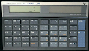
| Calculator App | Electronic Calculator | Slide Rule | |
| Basic | 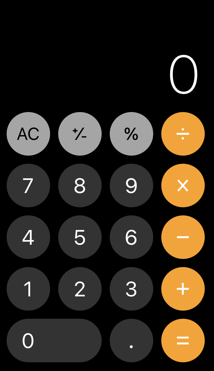 |
 |
 |
| Advanced | 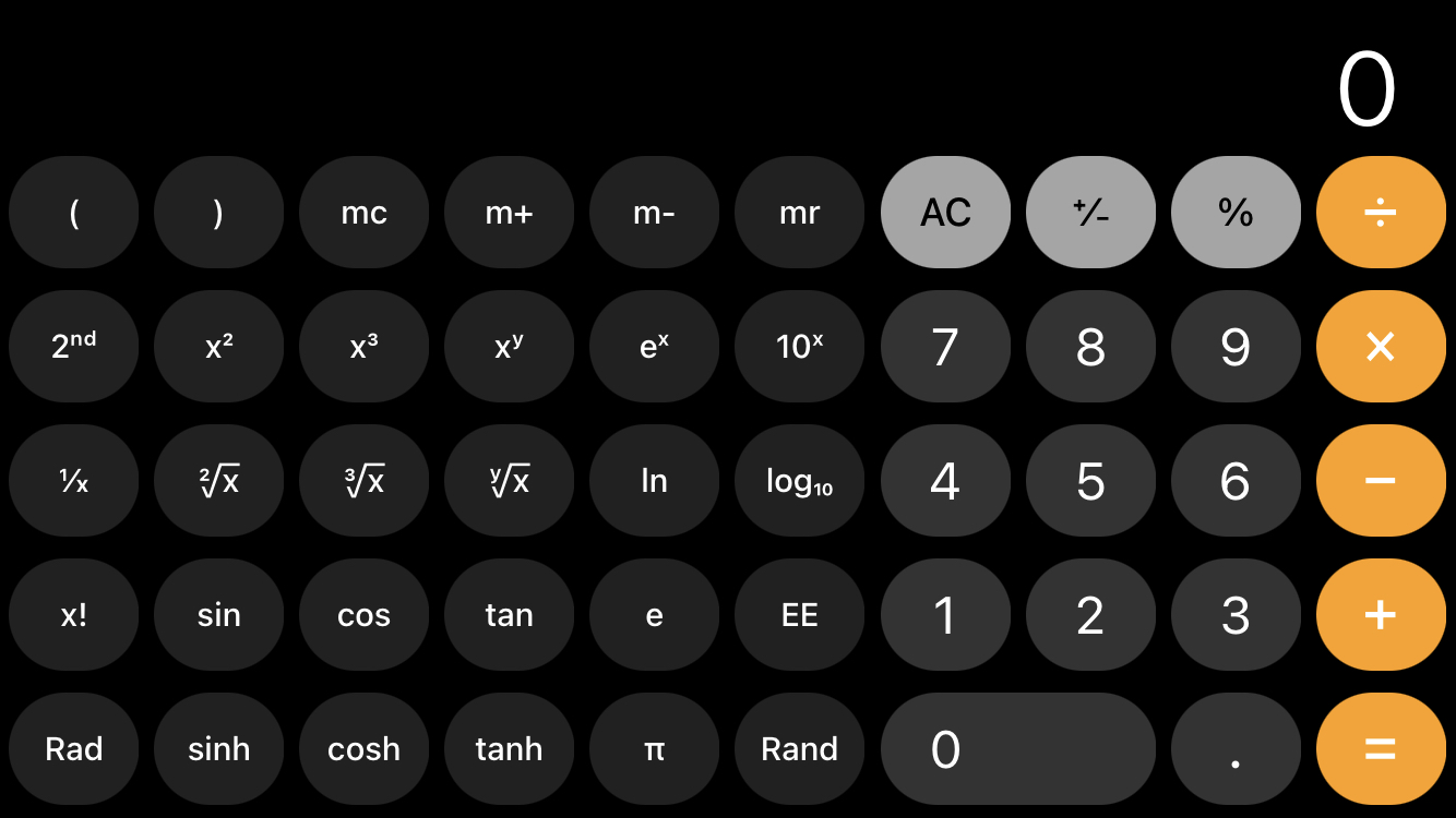 |
 |
 |
| 2010-? | 1975-2010 | 1624-1976 |
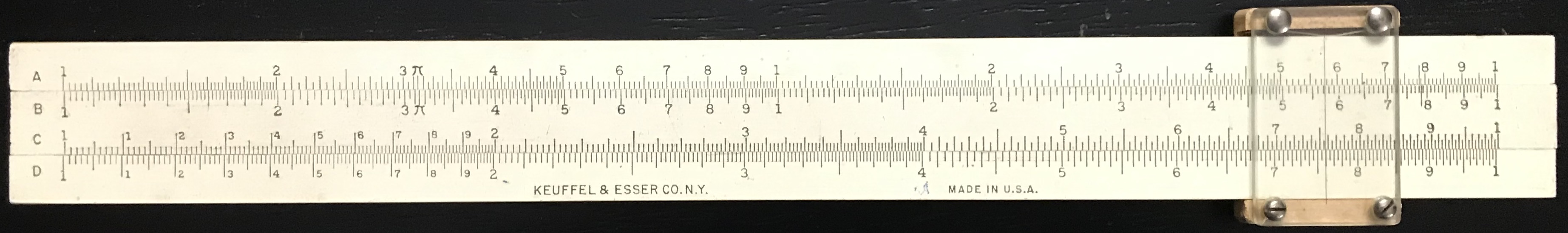
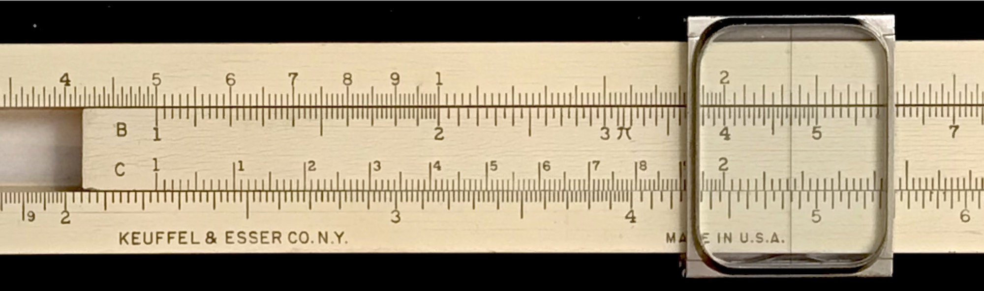
For a computational example, let’s calculate 5 times 4.7 using the A and B scales on a slide rule, such as the top two scales on the basic slide rule in the image above. Using the slide rule, we slip the indicator, or cursor, so that its hairline is over the 5 on the A scale. We then move the left-hand side of the slide (center section) to line up the 1 on the B scale with the hairline. We can then move the cursor’s hairline to 4.7 on the the B scale. The result is found beneath the hairline on the original A scale: 23.5. In fact, 5 times any other number can now be read from this single setting, as you can see below: 5 \(\times\) 1.5 = 7.5; 5 \(\times\) 2 = 10; 5 \(\times\) 3 = 15; 5 \(\times\) 4.5 = 22.5 (or, 0.5 \(\times\) 0.45 = 0.225), and so on. Many other standard operations and techniques for using the slide rule can be found in Chapter 3, and the mathematics behind their guiding principles can be found in Chapters 1 and 2.
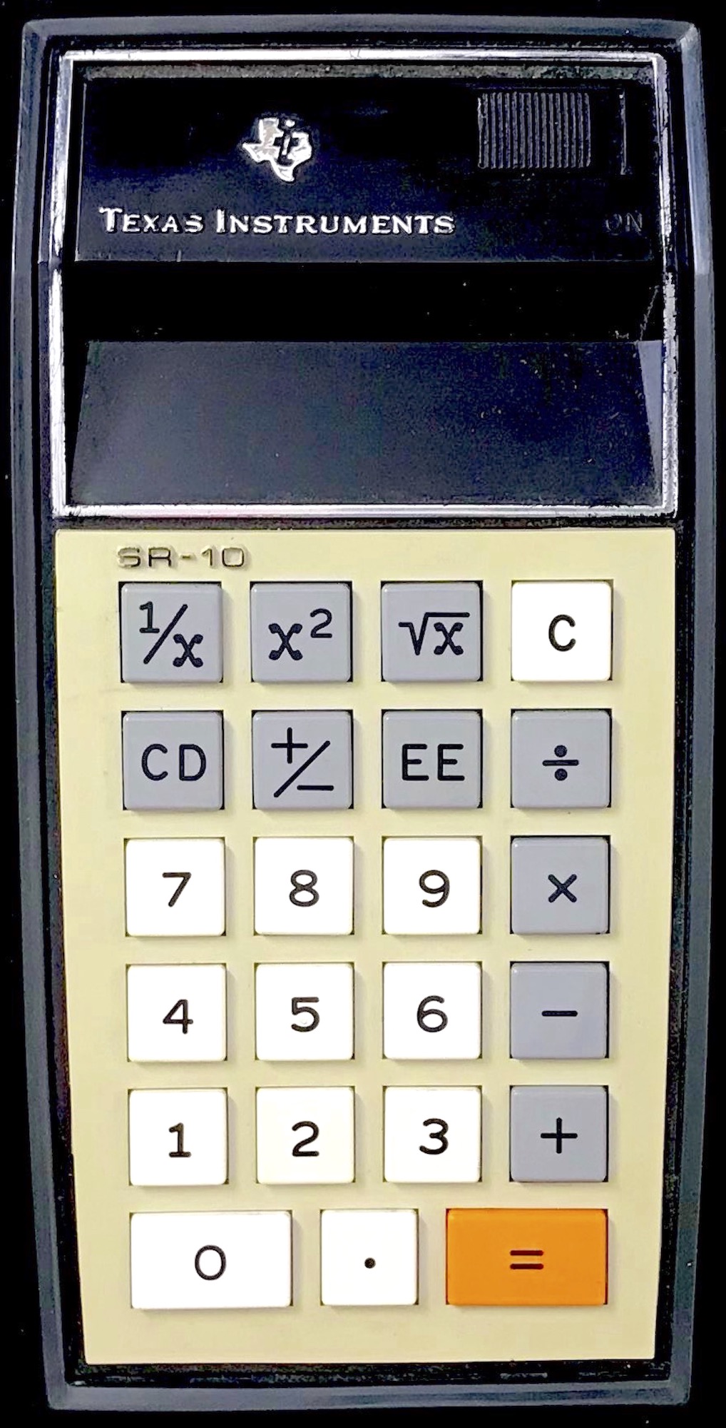
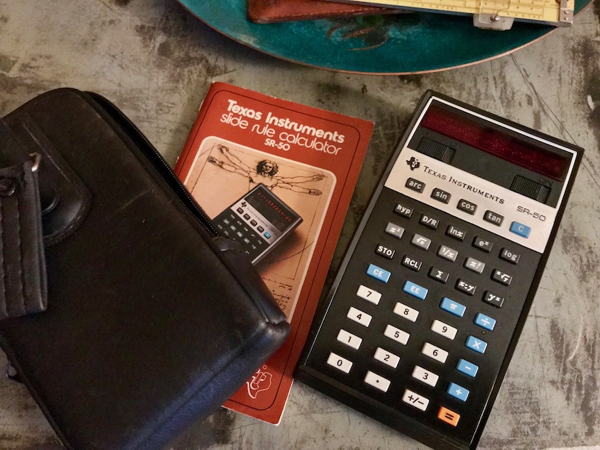
The earliest pocket electronic calculators that became affordable to the general public were sometimes named “slide rule calculators” to emphasize that they performed most of the same functions. Below is an image of my pocket calculator from college.
Early electronic calculators of the 1970’s were capable of performing numerical calculations with multi-digit (usually 10-13) precision; but for many computations, only 2-3 digit accuracy – or 4 at most – is sufficient for the project at hand. Note that an error in the last digit in a three-digit number is on the scale of 1 part out of a few hundred, say 1 out of 500 as an example; this amounts to an error of about 0.2% or so for a typical calculation. Computations necessary for the building of buildings and sidewalks, bridges and automobiles, even airplanes and rocket ships could be performed through the use of slide rules for many of the relevant calculations. Mechanical computing machines and other techniques could be used sparingly in special cases where more accuracy was critical.
For perspective, the bottom line in the image below is 0.2% longer than the top line:1

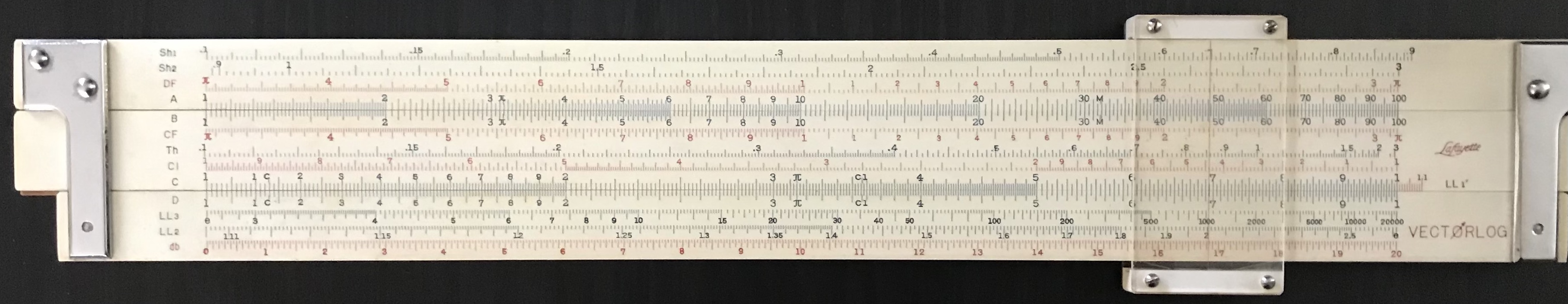
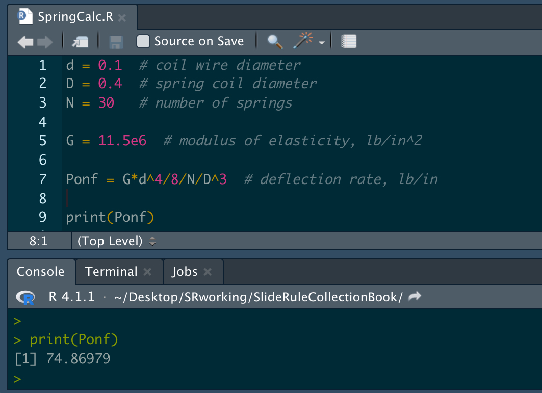
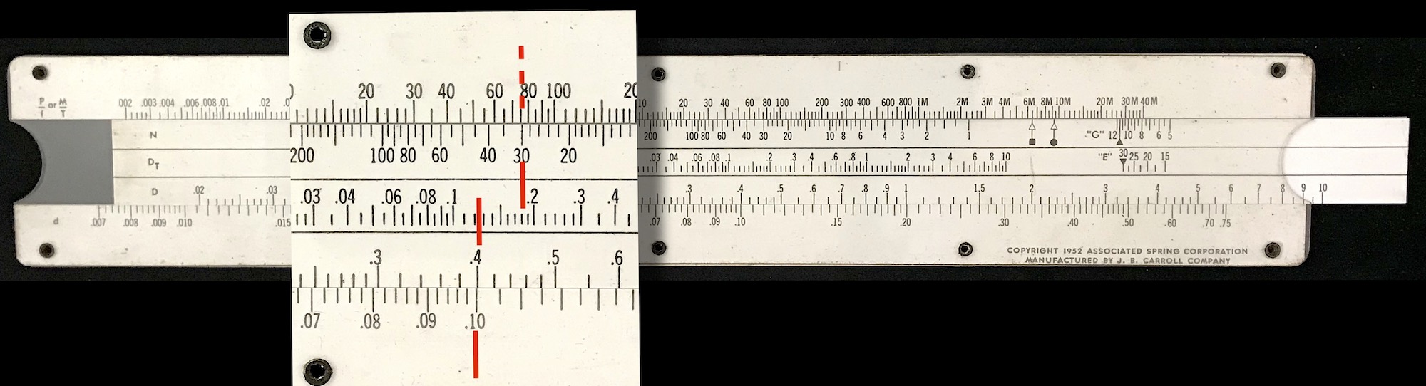
When calculations need to be repeated many times over, such as in design work or operations, computer programs and applications are very often used today. Prior to computers and programmable calculators, a wide variety of specialty slide rules permitted designers and other professionals to perform expeditiously such repetitive tasks. Our next image compares a small computer code that evaluates an engineering equation on a personal computer, and a slide rule from the 1950s that was designed to perform the same calculation. While such specialty slide rules had little practical application outside of their intended use, this also makes many of them rather rare and thus often highly collectible.
The development of the concept of a logarithm paved the way for the invention of a logarithmic scale, with which one could perform the multiplication of arbitrary numbers by adding or subtracting lengths along a physical rule. Following this invention in the early 17th century, additional scales were gradually created over time and added to the slide rules produced over the centuries so that more complex calculations could take place on these relatively simple and easy to carry devices.
The web site is divided into several parts – Organization, Review, and The Collection. Following our current overview of the site and its organization, the first three chapters present a review of the concept of logarithms and how logarithmic scales on slide rules allow for a wide variety of calculations. Then, with this information at hand, the next five chapters present in a variety of ways The Collection of slide rules and books. Before diving right in, our final introductory section will preview in more detail the various chapters, special sections, and other content that can be found on this web site.
To see the difference, note that the left ends of the two lines start at the same horizontal location on the screen. Using as large a monitor as possible, magnify the screen image and scroll the lines to the left side to verify that they can line up with the edge of the screen. Then, carefully scroll the image to the right side of the screen; you’ll find that when the bottom line touches the right side of the screen’s edge, there will be a small gap between the monitor edge and the upper line. It is 0.2% shorter.↩︎