8.31 An Early Home-Made Spring Calculation Slide Rule
Originally posted: 2021 Jul 01
See the article in the Jour. Oughtred Soc., V31.2p57 (2022).
During the pandemic of 2020 I found myself continuously drawn to an eBay advertisement for a “Vintage Wood Wooden Spring Weight Calculator Slide Rule”. The slide rule was reasonably priced, but appeared perhaps to be home-made, rather than manufactured by a major slide rule maker. On the other hand, it apparently had two distinct side-by-side slides on its front face, a feature I had seen in pictures before, but had not encountered first-hand. After watching the posting for several months, I finally purchased it for under $20 mainly to look at its use of two adjacent slides and also because it was literally just a few miles down the road from my home in Illinois. The on-line images were not very sharp and so it was hard to tell what all the scales were and, although an image showed otherwise, I had assumed it to be of length 10 inches or so. I was surprised when I got my hands on it and it was actually 17 inches in length. Talking to the antique dealer in Elmhurst, IL, she wasn’t sure where the slide rule came from – it was found in a box of items traded between dealers – and hence was not familiar with its history.
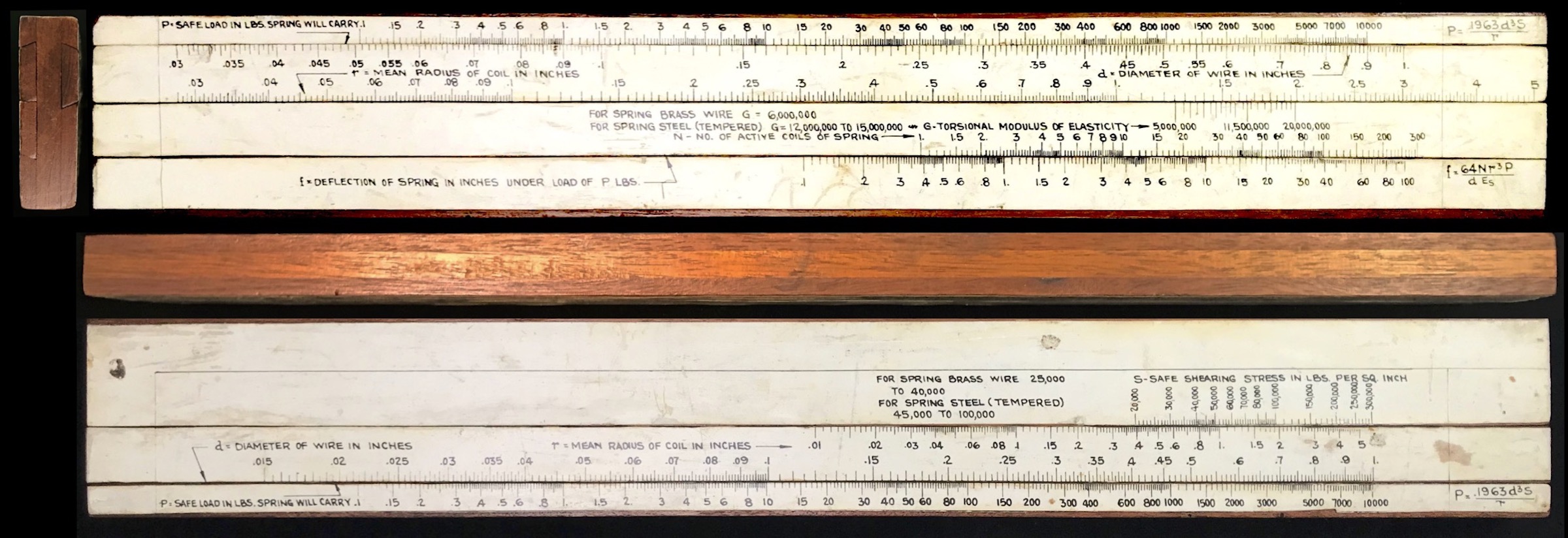
The stock of the slide rule is made from 3-ply plywood, 0.75 inches thick, with a total width of 2.5 inches. The device has no cursor. As noted, the front side of the rule has two side-by-side slides, while the back side also has a totally separate slide, thus three slides in all. The scales are on paper glued to the wood, and the scales and labels appear to have been written by hand, though rather professionally drawn. An image of the slide rule is shown below.

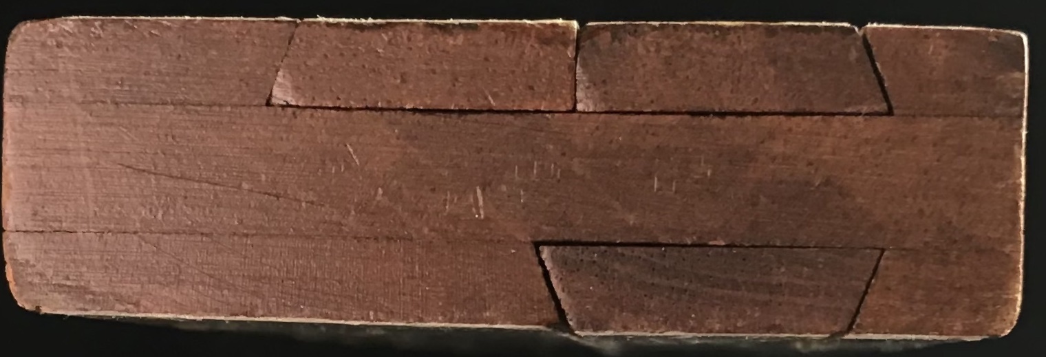
It is interesting that the slides of this apparent home-made rule have been cut from the stock in a dovetail fashion. The two adjacent slides have been formed by a single dovetail cut through the stock, and then a single square cut being used to form two pieces. This arrangement guarantees that these two slides only fit one way, yet stay snugly in place when the rule is turned over. A detail of the end of the slide rule is shown below.

From Michael Konshak’s comprehensive JOS article in 2006 JOS138, the earliest spring design calculators appeared as slide charts in the late 1940s, generated by companies that manufactured springs. (Recent communication indicates that this conclusion has not changed in the past 15 years.139) However, slide rules for such calculations were made by major manufacturers from 1952 and later, perhaps most notably by Pickett in Chicago, though spring slide rules by Acu-Rule Manufacturing Company in Mt. Olive, IL, (Acu-Math) are also mentioned in the article.
The slide rule at hand has scales that are used to evaluate the following two equations, which are written on the upper and lower stock of the rule:
\[
P = \frac{0.1963\;d^3 S}{r}
\]
and
\[
f = \frac{64 N P r^3}{d^4 G}.
\]
The slide rule has an error in the printing of this last equation (\(d\) rather than \(d^4\)), though the scales themselves perform the correct calculation. Additionally, I have used the symbol \(G\) above rather than \(E_s\) as shown on the rule, since closer inspection showed that the symbol \(G\) is used to label the relevant scale on the rule, rather than \(E_s\).
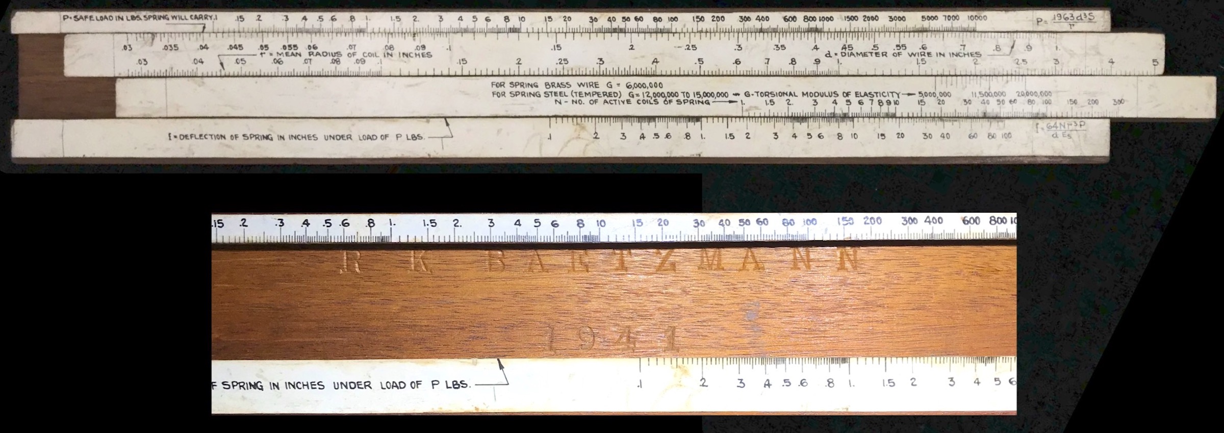
But most significantly, when I finally took out the slides to inspect the construction of the rule, I found engraved in the well of the front side:
R. K. Baetzmann
1941
The slide rule apparently pre-dates the earliest examples of the known slide rules and slide charts of this genre from the major slide rule and spring manufacturers.

8.31.1 R. K. Baetzmann
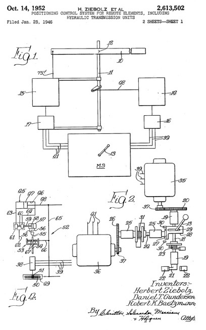
A simple on-line search revealed that Robert Kristian Baetzmann was born in 1908 and grew up in Chicago, Illinois. Records show that he studied Mechanical Engineering at the University of Illinois in Urbana-Champaign, graduating in 1932.140 The search also revealed that Mr. Baetzmann was a member of a three-person group that received a patent, submitted in 1946 and granted in 1952, for a positioning control system.141 The patent shows that Baetzmann was working at the Askania Regulator Company in Chicago at the time the patent was submitted. The lead author of the patent also of Askania is Herbert W. Ziebolz, one of the pioneers in the field of automatic control and who was responsible for many patents in such areas as jet pipe regulators and signal devices, translator chains, and pneumatic safety devices.142 (The third author, Daniel T. Gundersen, is known for his 1948 patent of the electric arc furnace control system.) Thus, it appears that Baetzmann may have been working for Askania at the time his slide rule was made.


Left: Cover page for 1952 Patent (filed 1946). Right: Excerpt from University of Illinois 1932 yearbook.
Following his work with Askania, Mr. Baetzmann was later employed for many years at the Metropolitan Sanitary District of greater Chicago and eventually retired from his position there. He passed away in Elgin, IL, in 2004. Beginning in 2005, the College of Engineering at the University of Illinois began to offer the Robert K. Baetzmann Scholarship for undergraduate study in various engineering disciplines.
8.31.2 Spring Calculations
A few of the more general parameters for basic spring design calculations involve the material being used, in particular its torsional modulus of elasticity, \(G\), and its safe shearing stress, \(S\); the diameter, \(d\), of the wire used in making the spring; the radius, \(R\), of each coil of the spring, and the number of coils, \(N\), used to make a complete spring.
With these parameters, one can compute the load \(P\), in pounds, that the spring can safely support, according to
\[ P = \frac{\pi}{16}\;\frac{d^3 S}{r}. \]
Additionally, one can compute the rate for the spring – the deflection of the spring per unit of load – or, alternatively, the deflection \(f\) directly through the relationship
\[ f = \frac{64Nr^3 P}{d^4 G}. \]
Slide rules constructed a decade or more later incorporated calculations of other design features and corrections (such as square vs. circular wire cross section, etc.). However, the early slide rule we have here is designed to analyze the two basic relationships shown above.
8.31.3 The Scale Set
The uncommon side-by-side double-slide front of the rule and the single-slide back side of the rule contain the following scales, using our above notation for the relevant variables:
| Front Scales | Back Scales |
| P [ d r ] [ G N ] f | S [ r d ] P |
where \(P\) is in pounds, \(d\), \(r\), and \(f\) are in inches, and \(G\) and \(S\) are in pounds per square inch (psi).
Each of the scales on the rule are logarithmic in nature, and a quick set of measurements provides the length of a decade on each. This scaling is slightly different on the two sides of the rule for values of \(r\) and \(d\) as shown in the following table:
| Front Scale | Range | distance on scale (over one decade) | Unit |
| P | 0.1 – 10,000 | ( 5.9 cm) \(\log P\) | lb |
| d | 0.03 – 1 | (23.6 cm) \(\log d\) = (5.9 cm) \(\log d^4\) | in |
| r | 0.028 – 5 | (17.7 cm) \(\log r\) = (5.9 cm) \(\log r^3\) | in |
| G | 5,000,000 – 20,000,000 | ( 5.9 cm) \(\log G\) | lb/in\(^2\) |
| N | 1 – 300 | ( 5.9 cm) \(\log N\) | |
| f | 0.1 – 100 | ( 5.9 cm) \(\log f\) | in |
| Back Scale | Range | distance on scale | Unit |
| S | 20,000 – 300,000 | ( 5.9 cm) \(\log S\) | lb/in\(^2\) |
| r | 0.01 – 5 | ( 5.9 cm) \(\log r\) | in |
| d | 0.015 – 1 | (17.7 cm) \(\log d\) = (5.9 cm) \(\log d^3\) | in |
| P | 0.1 – 10,000 | ( 5.9 cm) \(\log P\) | lb |
Let’s first look at the calculation performed on the back of the slide. The general formula is \(P = (\pi/16) d^3 S / r\) = \(0.1963\; d^3 S / r\), which can be re-written as \[ S/r = P/d^3\times 5.09. \] Matching up a value of \(r\) on the slide with a value of \(S\) on the stock is equivalent to finding \(S/r.\) Doing the same at the bottom interface, lining up numbers on \(d\) on the slide with numbers of \(P\) on the stock is taking the ratio of \(P/d^3.\) And, if \(P\) = \(d\) = \(r\) = 1, then, within factors of 10, we should find \(S\) = 5.09, and indeed this is the case. Lining up \(P\) = 10,000 with \(d\) = 1 we find that \(r\) = 1 is aligned with \(S\) = 50,900.
We thus have all that is needed to complete the slide rule configuration for this calculation. Values for \(S\) and \(r\) are paired at the top interface of the stock and slide, while \(P\) and \(d\) are paired at the bottom interface. Maximum reasonable ranges for the more important parameters, like \(r\) and \(d\), are determined and using a reasonable range for \(S\), the \((S,r)\) pair is placed at a convenient location on the rule. The overall markings are set by the overall factor of 5.09.
Looking at the front side, with two slides, the general formula has more factors, specifically \(f = 64 N r^3P/(d^4G)\) or, equivalently,
\[ f/N = (P/d^4) \times (r^3/G) \times 64. \]
A quick check on the slide rule can be made if we move the two slides such as to line up \(d\) = 1 on the top slide with \(P\) = 10,000 on the top stock \((P/d^4 = 10^4)\), then line up \(G\) = 10,000,000 on the bottom slide with \(r\) = 1 on the top slide \((r^3/G = 10^{-7})\). Doing so we find that \(f\) = 6.4 on the bottom stock is opposite \(N\) = 100 on the bottom slide and \(f\) = 0.64 is opposite \(N\) = 10, i.e., \(f/N\) = 0.064 (= \(64\times 10^{-3}\)) as required.
So, for this side of the slide rule, \(P\) and \(d\) are paired at the top interface, while \(r\) and \(G\) are paired at the second interface and \(N\) and \(f\) are paired at the third (bottom) interface. Maximum reasonable ranges for the important parameters, like \(r\), \(d\), \(P\), and \(f\) are used to set the overall extent of the scales, and likely helped to determine the overall length of the slide rule itself. Selecting reasonable ranges for \(G\) and \(N\), the \((r,G)\) and \((N,f)\) pairs can be positioned at convenient locations on the rule.
8.31.5 Final Remarks
Our example here is a very early spring design calculation slide rule, the earliest dated example that I’ve been able to find through online searches and communications with contacts. Its unique 3-slide feature made from a single stock makes it especially interesting as an example of a multi-parameter calculation device.
In creating and/or overseeing the manufacturing of his slide rule, Robert Baetzmann of Chicago was perhaps influenced by the city’s local slide rule companies such as Post, Dietzgen, Keuffell and Esser, and others who had headquarters and other major offices in the city. Or, perhaps it was the other way around. As an engineer working for metropolitan Chicago, it begs the question as to whether Baetzmann had early interactions with the slide rule makers in town, particularly Pickett, whose model 1025 came on the scene within a few short years after Baetzmann’s rule.143 Our early slide rule could very well have been a concept that was presented to one of the slide rule companies that soon enticed the manufacturer to produce spring design models. On the other hand, it might be that Baetzmann found it easier and more satisfying to simply “build his own” slide rule, and that’s that.
Whatever the story behind the man, the Baetzmann slide rule is a great piece of history, showing that spring design calculations had become commonplace enough to demand their own special slide rule in the early 1940s, and demonstrating what a good Midwestern engineer will do to get the job done. (No bias here, of course.)
Michael Konshak, “The Spring Design Slide Rule Calculator”, J. Oughtred Soc. V15.1 p28 (2004).↩︎
Michael Konshak, private communication.↩︎
See The Illio 1932 yearbook; https://archive.org/details/illio193239univ/mode/2up.↩︎
United States Patent Office, No. 2,613,502, “Positioning Control System For Remote Elements, Including Hydraulic Transmission Units”, Herbert Ziebolz, Daniel T. Gundersen, and Robert K. Baetzmann, Chicago, IL.↩︎
See On Herbert W. Ziebolz, Transactions of the ASME, March 1975, p.4.↩︎
See Konshak JOS article above.↩︎
8.31.4 Comments on Accuracy
A close inspection of some of the lines marked on the slide rule provides evidence of a hand-drawn system and questions the accuracy of the device. If the distance between decades along a logarithmic scale is \(L_0\), then the value \(x\) on the scale is a distance \(L = L_0\log x\) = \((L_0/\ln 10)\ln x\). An error \(\Delta L\) in the printing/reading/setting of a mark on the rule will give an error in the value of \(x\) provided by \(\Delta L\) = \(L_0/\ln 10\) \(\cdot\) \(\Delta x/x\), and so the error in the calculation \(\Delta x/x\) will scale like \[ \frac{\Delta x}{x} = \frac{\ln 10}{L_0}\cdot \Delta L. \] For the hand-drawn lines on the Baetzman slide rule, the length of the standard decade is \(L_0\) = 59 mm, or \(\Delta x/x = \Delta L/(25.6~{\rm mm})\) for this rule. A marking error of, say, 0.5 mm or so would give an error in the evaluation of \(x\) of about 2%.
It’s easy enough to check the computations of the slide rule against modern technology. Let’s first check the back side calculation. Taking \(S\) = 200,000 and \(r\) = 0.3, let’s compute \(P\) for values of \(d\) = 0.02, 0.08, 0.25, 0.35 and compare to using the slide rule. When I use the slide rule for these combinations of numbers I get: \(P\) = 1, 66, 2000, 5500. The results using a computer are: \(P\) = 1, 67, 2044.8, 5610.9. This gives a typical error of about 2.5%.
Repeating the above, but with \(S\) = 30,000, gives a typical error of about 1.9%.
On the front side, we have more variety in the parameter combinations, but let’s try a similar exercise. Let’s use values of \(P\) = 9 and 1500, and take \(d\) = 0.32. Suppose \(r\) = 1. Using \(G\) = 8,000,000 and 18,000,000 we’ll compute \(f\) for values of \(N\) = 40 and 150. The results are shown in the table below.
Results for \(d\) = 0.32, \(r\) = 1:
Neglecting the case that went off-scale, the typical error in the above calculations compared to a computer-generated result is 2.5%.
Overall, while an exhaustive error analysis of the slide rule accuracy was not performed, it is clear that typical calculations on the rule are expected to be accurate to the few percent level which is arguably consistent with a hand-drawn system.