8.34 Stadia Rules
Latest Update: 2024 Dec 01
Originally posted: 2022 Jan 05
Slide rules for use in the field or office were standard tools for the surveyor. And specialty slide rules, with specific scales for use in tacheometric – or, stadia-metric – calculations, were sold by several manufacturers. The stadion is a unit of distance from ancient Greece, on the scale of about 600 feet or about 190 m, and a stadia measurement is a method to rapidly determine horizontal and vertical distances, typically on the scale of the stadion, using a telescope (usually a surveyor’s transit or a theodolite) and a vertical graduated rod. If you’ve ever seen a surveyor at a telescope on the side of the road, with a partner down the way holding a tall rod with markings on it, this is what they were doing.
8.34.1 The Stadia Measurement
An optical telescope will have a “field of view” for a particular set of optical focal lengths and eyepiece style. A good transit telescope might have an objective lens of about 2 inch diameter or less, and perhaps a focal length of about 12 inches or less. Typical magnification might be about 40x. Only a certain cone of light rays can enter the objective lens and become focused through the eyepiece onto the observer’s retina; the angular divergence of this cone would be the field of view.
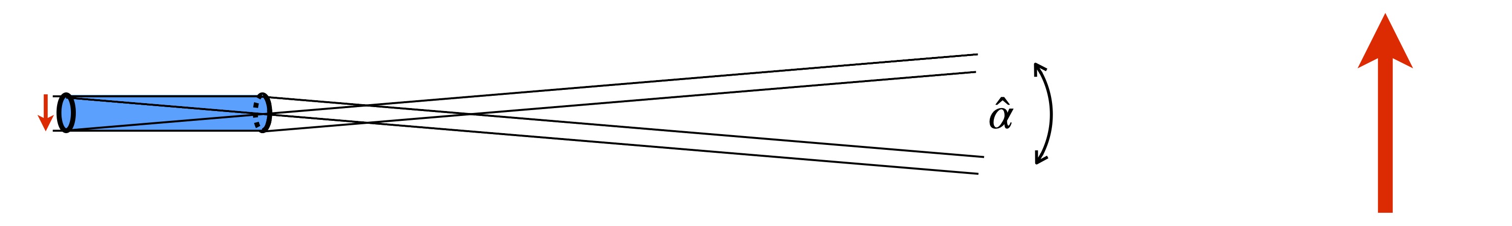
To get a rough scale of the effect, imagine an object located far away (“at infinity”) from the telescope for which we wish to form a primary image the size of the telescope’s diameter. With the tube of the telescope being approximately the length of the objective lens’ focal length, the total field of view \(\hat\alpha\) should be approximately
\[ \hat{\alpha} \approx D/F \approx (2~{\rm inch})/(12~{\rm inch}) \approx 0.17~{\rm radian} = 170~{\rm mrad}, \] or about 10 degrees for the parameters given above. However, the actual result will depend upon properties of the eyepiece of the telescope being used as well, which results in a much smaller overall field of view.
Eyepieces, which typically use multiple shorter focal length lenses, will have correspondingly larger fields of view, perhaps \(\alpha_e\) = 45-70\(^\circ\) or so. However, the magnification of the telescope, given by \(m = F/f_e\) where \(f_e\) is the eyepiece focal length, will reduce the field of view of the telescopic system by this factor:
\[ \hat\alpha = \alpha_e/m = \alpha_e\times f_e/F. \]
Thus, a magnification of about 40x would give an overall field of view of about 1-2\(^\circ\), or about 15-30 mrad, for instance. Suffice it to say, the scope used as a tacheometer will have a field of view on the scale of a small number of degrees, or tens of milliradians.
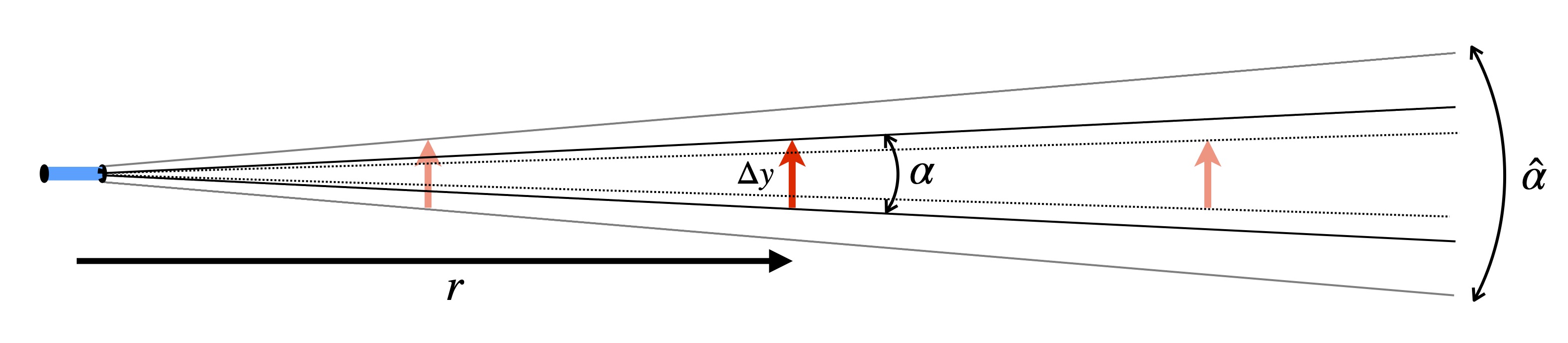
With a fixed field of view, an object of fixed size \(\Delta y\) will appear proportionally smaller through the telescope when viewed at larger distances \(r\), as illustrated below.
For use as a transit telescope, markings on the optics of the telescope provide a view to the user of lines that mark angular measure, or stadia lines, such as at \(\pm\) 5 mrad, for instance.
Now imagine one aimed the telescope at a vertical rod off in the distance, and that the rod had markings of feet and inches along its length. If through the telescope the user views the upper and lower stadia lines (at \(\pm\) 5 mrad) going across marks on the rod that are known to be separated by 12 inches (one foot), then the rod must be located approximately 100 feet away.
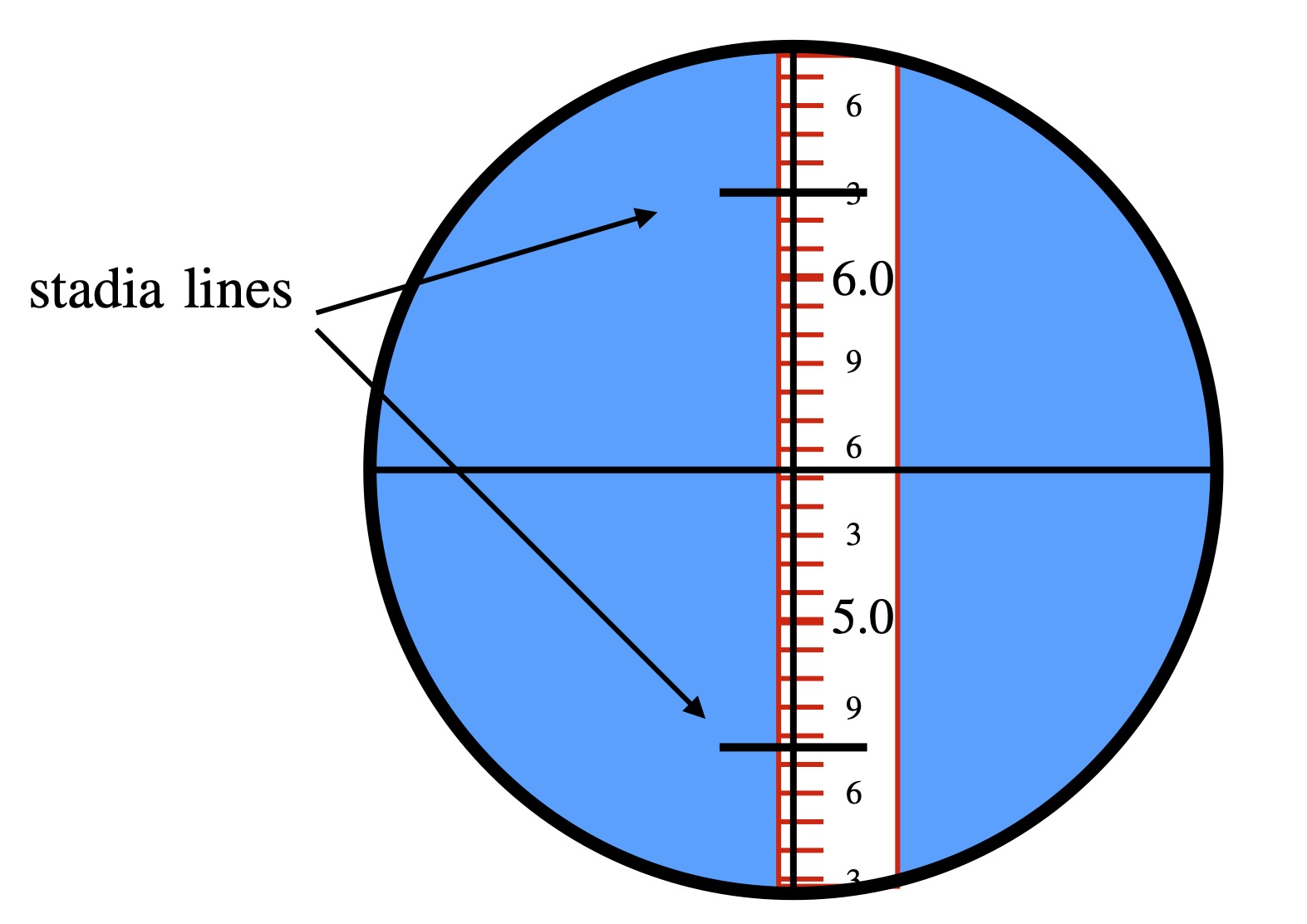
Suppose \(\alpha\) is the total angle between two stadia marks visible through the telescope. The vertical distances are read along the rod which cross the upper and lower stadia lines at \(\pm\alpha/2\) = 5 mrad.
- subtract the two readings to give total vertical distance between the two, that is, the distance visible within the angle \(\alpha\).
- multiply by 1/(\(\alpha\)) = 1/0.010 = 100 to get the actual distance to the central measurement point.
Note that when more accuracy in the distance is required, particularly for closer objects, surveyors would typically use a chain or tape to measure the distance directly if possible.
8.34.2 Horizontal Displacement and Vertical Rise
So far we have only been discussing the direct distance to the object from the telescope. However, the object might be at a different elevation than the transit. So what we really want is the level horizontal distance to the object’s location as well as its elevation relative to the transit. A collection of such readings and calculations would produce a topographical map of the area.
Presume the surveyor is using an instrument with stadia marks \(S1\) and \(S2\) visible through the telescope and separated by an angular field of view of \(\alpha\). A typical measurement might go something like this:
- transit is located on one level, distance \(t\) above grade
- the stadia rod, located at a higher elevation, has a measurement point \(M\) also a distance \(t\) above grade (If not exactly \(t\), can make necessary correction in the calculation.)
- the transit is aimed at \(M\); surveyor records lower/upper distances \(y_1\) and \(y_2\) on the rod, at stadia marks \(S1\) and \(S2\) as seen in the transit; compute \(\Delta y = y_2-y_1\)
- the direct distance \(r = (1/\alpha)\times \Delta y = 100 \times \Delta y\) is computed
- the transit angle \(\theta\), which is found on the telescope mount, is recorded
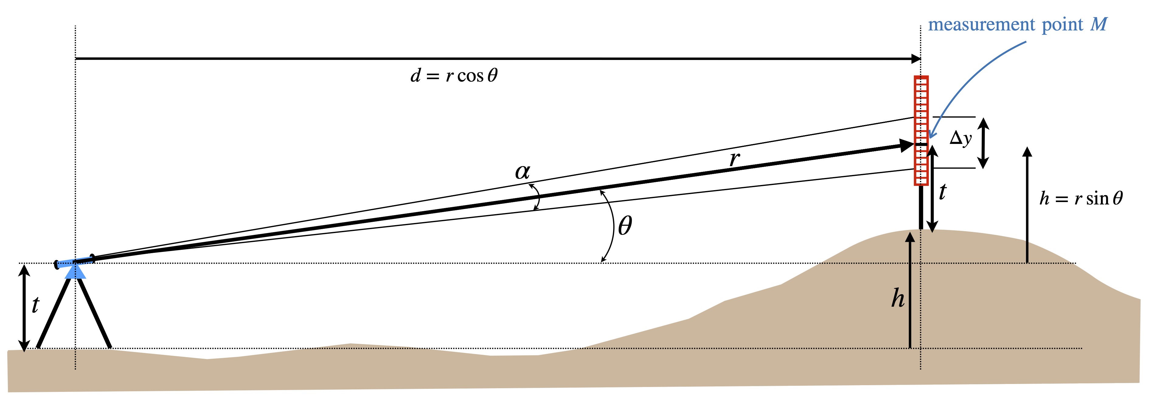
When viewing the stadia rod measurement point at an angle \(\theta\), the distance to the upper reading on the rod will be slightly different from the distance to the lower reading on the rod. A close up of the measurement point on the stadia rod is illustrated in the figure below:
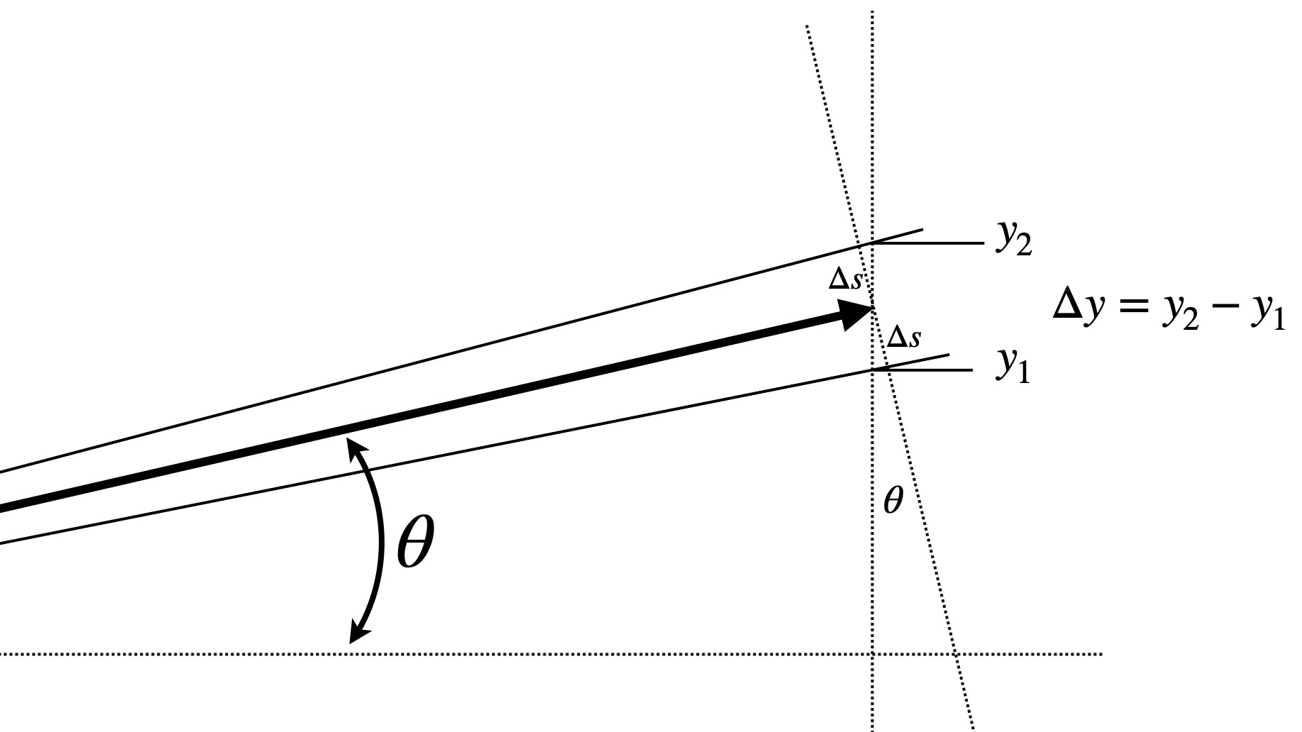
From this figure, we can see that
\[ \Delta s = r\times(\alpha/2) \] and \[ \Delta s = \frac{\Delta y}{2} \;\cos \theta. \] So, \[ r \times \alpha = \Delta y \;\cos \theta \] from which \[ d = r \cos \theta = \frac{\Delta y}{\alpha} \;\cos^2 \theta \] and similarly, \[ h = r \;\sin \theta = \frac{\Delta y}{\alpha} \;\cos \theta \sin \theta. \]
We see that while standard slide rules have standard trigonometric scales, new scales for computing \(\cos^2\theta\) and \(\cos\theta\sin\theta\) (which is also equivalent to \(\frac12\sin2\theta\)) would be very useful for quick in-the-field survey calculations, and these are what the stadia slide rules provide.
8.34.3 Stadia Slide Rule Scales
The basic stadia slide rule will invoke multiplications of the quantities \(\cos^2\theta\) and \(\cos\theta\sin\theta\), so let’s plot these functions:

If \(\theta\) = 0, then the measurement would be perfectly horizontal, and the elevation change \(h\) would be zero while the distance \(d = r\). For a measurement with \(\theta\) = \(45^\circ\) we would have \(h = d\). If \(\theta\) were \(90^\circ\), the horizontal distance would be zero – we would be measuring something directly above us. And, accordingly, as \(\theta\) approaches \(90^\circ\) the stadia marks visible through the transit would become harder and harder to discern. So such large angles on the slide rule would be meaningless. The range of practical angles is typically taken to be between 0 and 45 degrees. Note also that since \(\cos45^\circ = \sin45^\circ\) = \(\sqrt{2}/2\), the two curves cross at a value of 0.5 for \(\theta = 45^\circ\).
So, let’s re-make our plot but switching the axes, using a logarithmic scale on the horizontal axis, and using angles between zero and \(45^\circ\) on the vertical scale. Note:
- if H = \(\cos^2\theta\), then \(\theta = \cos^{-1}(\sqrt{H})\).
- if V = \(\sin\theta\cos\theta = \sin(2\theta)/2\), then \(\theta = \sin^{-1}(2V)/2\).

The horizontal spacing between the vertical hash lines in the plot above give the spacing of the five-degree markings on the major angular scale on the slide of the stadia rule, where the main axis shown would be represented by an A scale (i.e., two decades, from 0.01 to 1.0) on a standard slide rule:
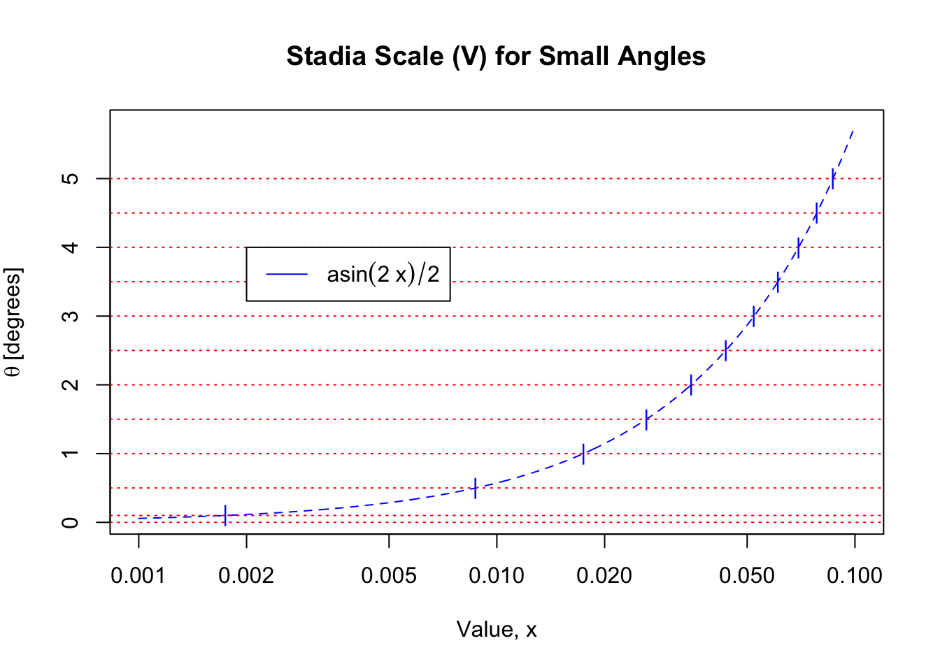
There also can be a separate scale on the slide for use when small angles are involved. For small angles, the cosine-squared quantity is assumed to be equal to one. So we simply repeat the cosine-times-sine calculation but for values 0.001 \(\lt x \lt\) 0.1, here indicated at half-degree intervals:

The markings on the slide of the rule would look something like this:

8.34.4 A Stadia Rule Example
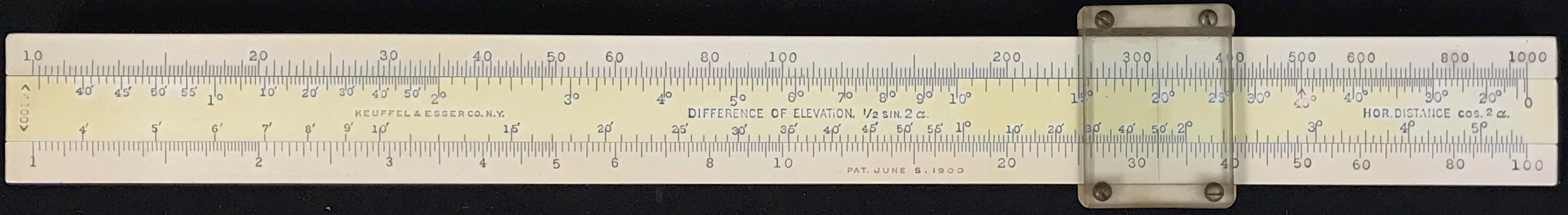
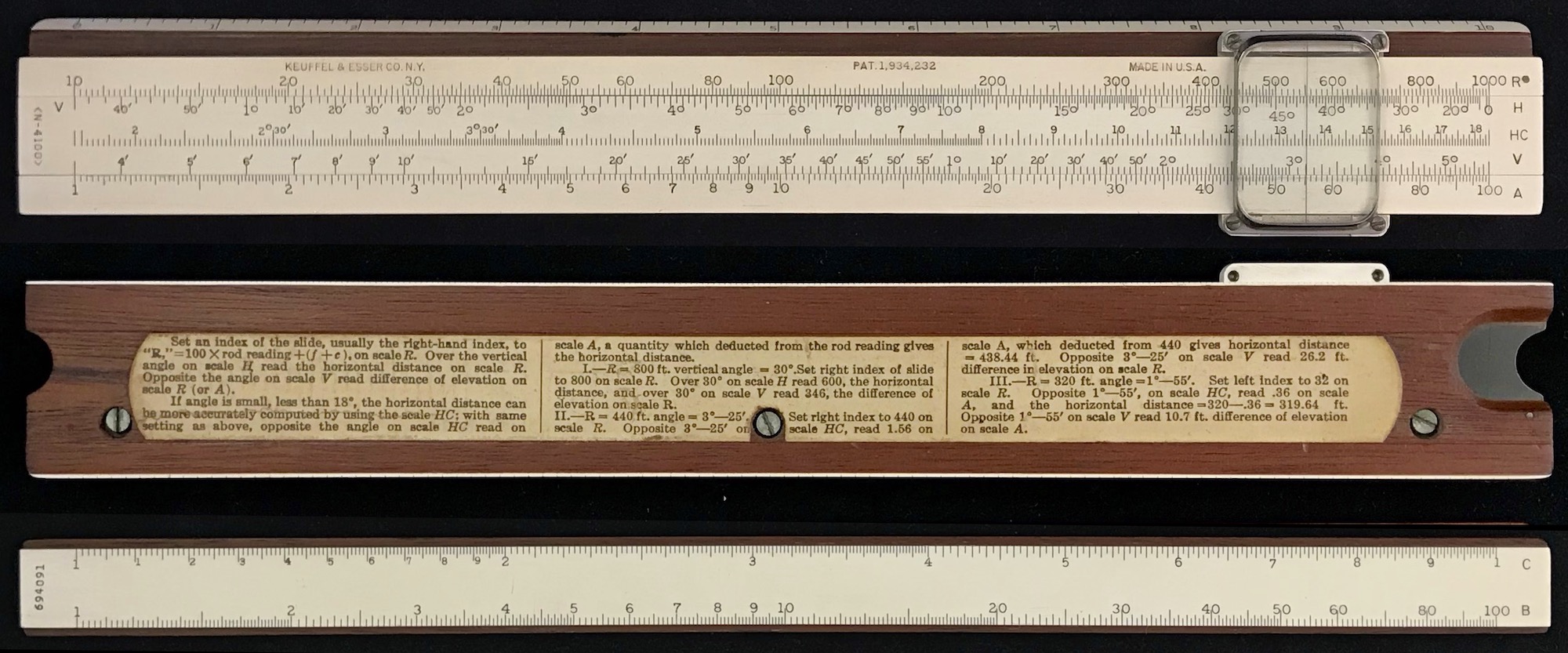
The example of a stadia slide rule from the collection is the Keuffel and Esser Model 4100, manufactured in about 1915-1922 and shown in the image below. The main scale, found on the lower stock, is an A scale, from 1 to 100. On the upper stock one finds a similar scale, often called the R scale where R = 10 \(\times\) A, which is labeled from 10 to 1000. The R scale is used to select the overall distance \(r\) in our discussions above. Notice that the left-hand side of the upper scale overlaps with the right-hand side of the lower scale.
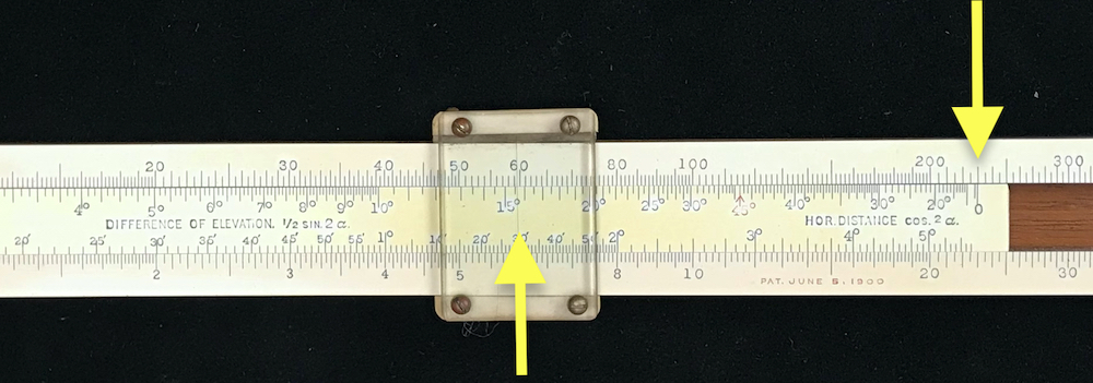
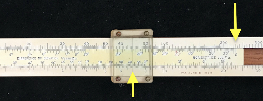
Next, on the slide we have two scales of angles, which correspond to the last two plots discussed above; the upper scale on the slide is for angles between about 0.5 degrees and 45 degrees, while the lower scale on the slide is for angles between about 3 minutes of arc to about 5.5 degrees, as in our last graph above. Note the red \(45^\circ\) mark on the upper scale of angles. To the left of this mark the angles correspond to the \(\cos\theta\sin\theta\) calculation; to the right of this mark, the angles are for \(\cos^2\theta\). The lower scale of angles is for small angle elevation calculations only.
To use the slide rule, the cursor is moved to a distance \(r\) on the R scale. Then the slide is moved to the left to line up the zero on the right-hand-side with \(r\). To find the horizontal distance \(d\), the cursor is moved to the value of \(\theta\) on the right-hand-side of the slide (to the right of the “45 degree” mark), hence multiplying by cosine-squared. The answer will be read on R at the cursor. For the change in elevation, \(h\), the cursor is moved to the same value of the angle, but to the left of the “45 degree” mark. If the angle is off scale to the left, then the angle is found on the lower scale on the slide, and the result is read on the A scale.
Example:
Suppose a measurement is made using \(\alpha\) = 10 mrad = 1/100, in which it is found that \(\Delta y\) = 2.3 feet at an angle of \(\theta\) = 15.6 degrees. Then,
- Compute \(r = \Delta y/\alpha\) = 230 feet
- Line up the zero on the slide with the value of \(r\)
- Move the cursor to the value of \(\theta\) to the right of the 45-deg. mark
- Read the value of horizontal displacement under the cursor on the R scale
- H = \((\Delta y/\alpha) \cos^2\theta\) = 213 feet
- H = \((\Delta y/\alpha) \cos^2\theta\) = 213 feet
- Move the cursor to the value of \(\theta\) to the left of the 45-deg. mark
- Read the value of the vertical displacement under the cursor on the R scale
- V = \((\Delta y/\alpha) \cos\theta\sin\theta\) = 59.6 feet
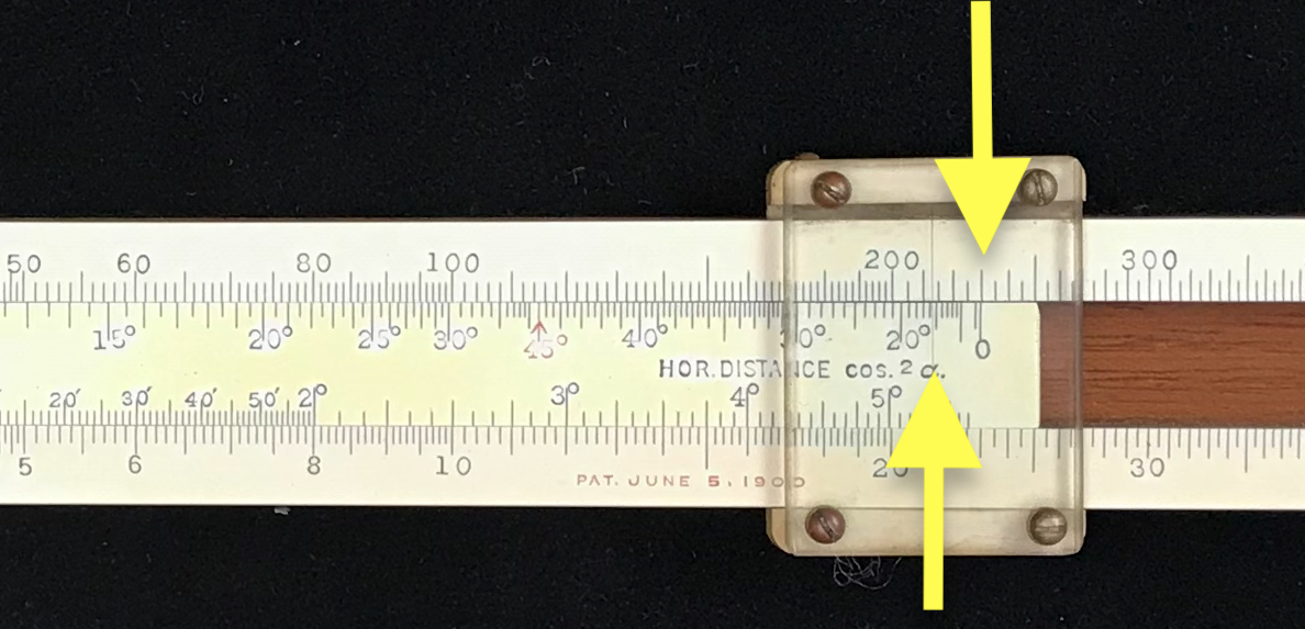 |
 |
Left: H calculation, right of \(45^\circ\) mark. Right: V calculation, left of \(45^\circ\) mark.
Now suppose instead that the angle was 1 degree 43 minutes. In this case,
H = \((\Delta y/\alpha) \cos^2\theta\) = 230 feet (Note: rule not used; H = \(r\) = \(\Delta y/\alpha\))
V = \((\Delta y/\alpha) \cos\theta\sin\theta\) = 6.9 feet (using lower scale)
8.34.5 Stadia Rule Variations
The stadia rule used above was the earliest rule of this type produced by Keuffel and Esser, the 4100. This model was first advertised in the K&E catalog in 1906, but in 1925 a new version – the N4100 – was revealed. This new stadia rule had the same scales, but with an additional scale on the slide to be used to determine horizontal distances when small angles (less than \(18\circ\)) are involved. On the original 4100, an additional “A” type scale (1-100) was included on the back of the slide; when the slide was reversed it could be used with the “A” type scale on the bottom of the rule for performing standard multiplication and division calculations. The N4100 added a standard “C” type scale (1-10) on the back of the slide thus allowing quick computations of square roots, for instance. The N4100 also added inch and centimeter scales on the edges of the slide rule.

About the same time that K&E was producing their first stadia rules in the U.S., another American company, Kolesch and Company in New York, was selling slide rules including a stadia rule as shown in the figure below.
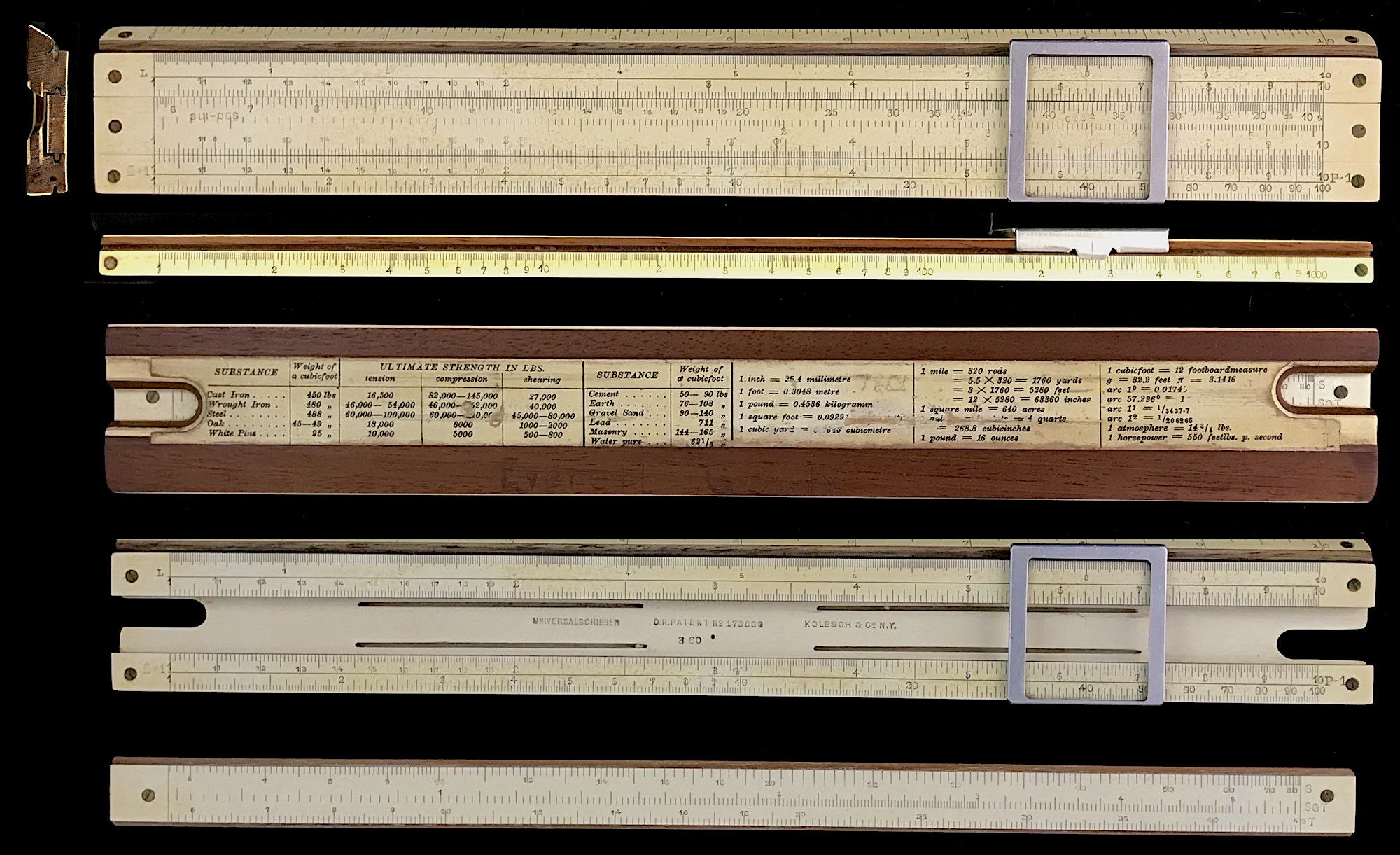
For this rule, a similar scale of \(\sin\theta\cos\theta\) and \(\cos^2\theta\) is present at the top of the slide, but only extends from values of 0.1 to 1, which is read from the standard C/D scales. Note that a D scale exists on the top of the stock next to the stadia scale. For interpreting values of \(\sin\theta\cos\theta\) between 0.01 and 0.1, a second stadia scale is present on the slide below the first. Though the rule has “Kolesch & Co N.Y.” engraved in it, the style of construction and application of German patents is indicative of Albert Nestler.
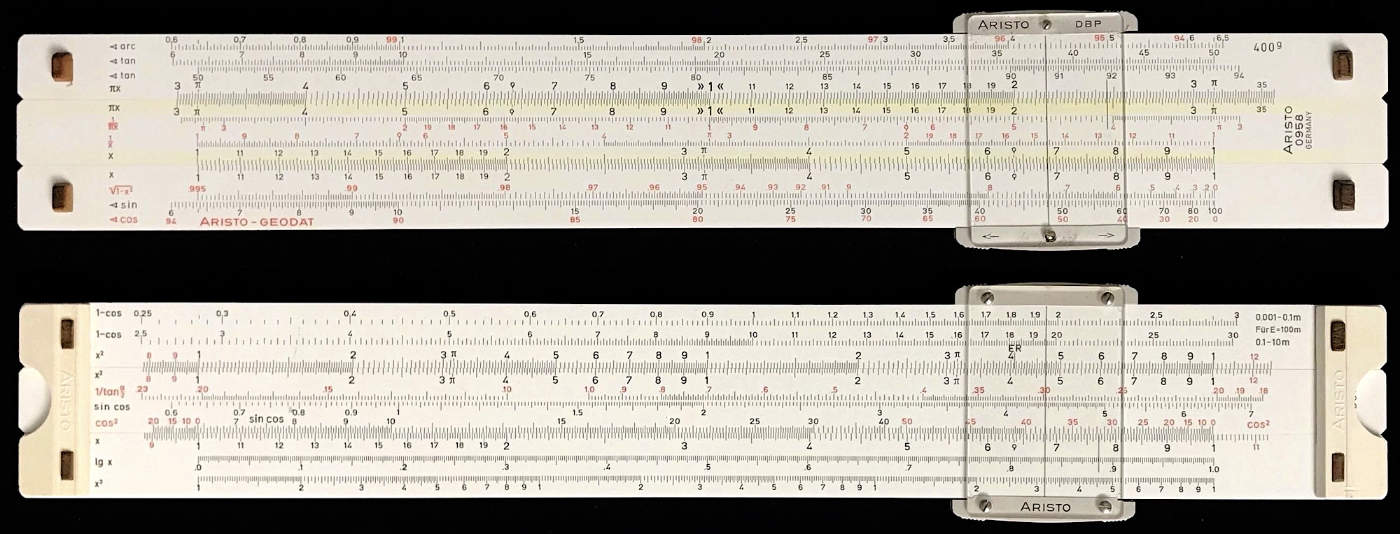
One of the more sophisticated stadia rules being used at the end of the slide rule era was the Aristo Geodat Model 0958. The front of the 0958 has 12 standard scales found on many slide rules for performing standard mathematical calculations, including trig scales and a P scale. On the back of the 0958 are another 10 scales. Besides C, A, B, K, and L scales, there are stadia scales that include:
- \(\cos^2\theta\)
- \(\sin\theta\cos\theta\)
- \(1/\tan(\theta/2)\)
- \(1-\cos\theta\) (two scales to cover two decades)
Aristo made two versions of the slide rule, one where the angles on the rule were in units of degrees, but also another version where the angles are written in units of the gon (or, grad or gradian or grade). The gon is a metric-centric measure of angle, where a right angle is made of 100 gon, which is equal to 90 degrees. The gon is not used in the U.S. but is still used by many surveyors in Europe. A version of the Aristo 0958 with gon as the angular unit is shown below. As in the (presumed German made) Kolesch rule, the angles on the Aristo are taken opposite a standard C scale from 0.1 to 1 or 0.01 to 0.1, providing a bit more accuracy in the readings, and allowing much more flexibility in the slide rule’s use for other calculations. In the image below, note how the bottom scale on the slide, labeled \(\cos^2\) in red, changes from a \(\sin\cos\) scale (in black numbers) to a \(\cos^2\) scale (in red numbers) at an angle of \(50^g\) (= \(45^\circ\)). The scale above this one, labeled \(\sin\cos\) (in black), gives the angles for the next lower decade in values found on the C scale, thus corresponding to the lower decade on the A scale of the K&E.
The figure to the right indicates relationships between angles and quantities found on the special scales of the geodat rule. |
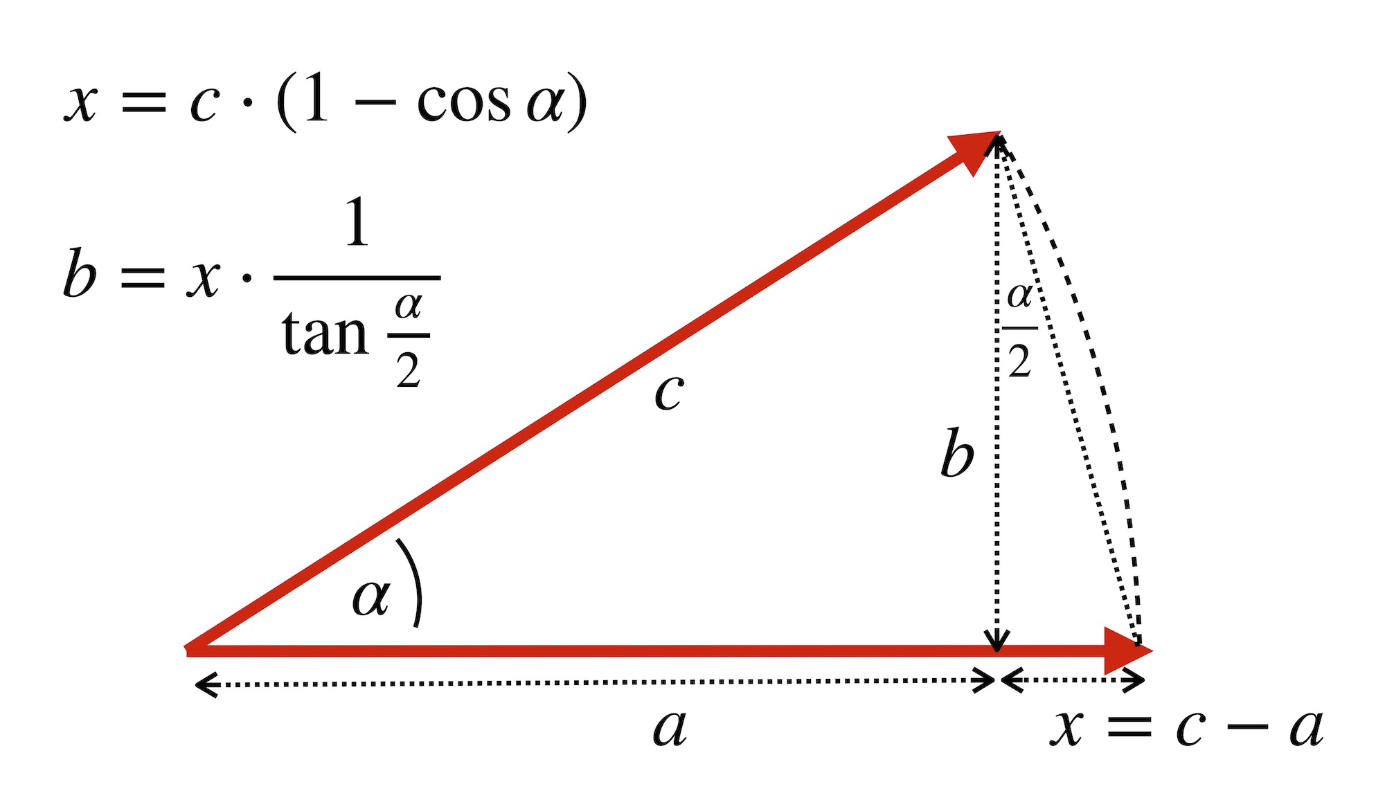 |
The instructions that came with the Aristo 0958 provide a very good explanation of all of these scales and their use, and can be viewed here (courtesy Peter Lang, via IRSM).
Further reading:
- The 50 Centimetre Slide-Rule as applied to Tacheometry and Curve-Ranging, with Tables, T. Graham Gribble, Cambridge 1911.
- Stadia or Tachymetrical Slide Rules, O.E. van Poelje, UKSRC Gazette No.6, 2005. I