8.33 Helical Slide Rules
Originally posted: 2021 Dec 12
The accuracy of a result on a slide rule is generally gauged by the length of the main scale on the rule. The longer the main logarithmic scale with numbers from 1 to 10, the more intervals can be marked and labeled between integers and the easier it is to read values and to interpolate between markings. A standard linear slide rule has a main logarithmic scale from 1 to 10 of length 25 cm (about 10 in) and gives results with a typical accuracy of about 0.1%. (See the vignette The Long and Short of It.) While longer linear slide rules were common, particularly of length 50 cm, further gains in scale length were made using circular, spiral, and helical scales.
Consider a linear scale of length \(d\). A circular scale of diameter \(d\) will have a total path length of \(\pi d\), or approximately \(3d\). Next, consider a spiral that has \(N\) turns going from a diameter of 0 to a diameter of \(d\); its total path length will be (very approximately) the sum of the circumferences of \(N\) circles of increasing diameters \(d\times n/N\), where \(n=1,\ldots N\). Its total path length will then be approximately
\[ s = \pi d\;\times \sum^N_{n=1} \frac{n}{N} = \frac{\pi d}{N} \; \times (1+2+\ldots+N) = \frac{\pi d}{N} \;\times \frac{N(N+1)}{2} = \frac{\pi d}{2} (N+1). \]
For example, if \(N\) = 10 this yields a path length of \(\frac{\pi}{2} d\times 11\) \(\approx\) \(17 d\). Now, consider a cylinder of diameter \(d\) and a helical curve wrapped around the cylinder. If the helix is tightly wound, then the path length of a helix made up of \(N\) windings will be approximately \(\pi d N\). Here, if \(N\) = 10, this yields a path length of about \(30d\).
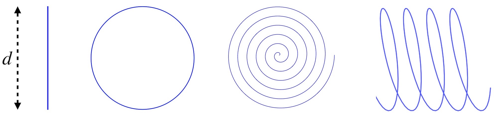
Note that for a given diameter, a spiral is constrained by the diameter of the disk. If a helix is drawn on a cylinder, then each turn of the helix has the same path length and the overall length is dictated by the diameter of the cylinder and by the length of its long axis.
Let’s look at a helix drawn on a cylindrical surface. Let \(r\) be the radius of the cylinder, \(h\) is the total length of the cylinder’s axis, and \(\theta\) is the angle of rotation about that axis. The number of rotations of the helix along it length is \(N\). That is, each rotation about the axis advances \(z\) by a value of \(h/N\). The configuration is illustrated in the figure below.
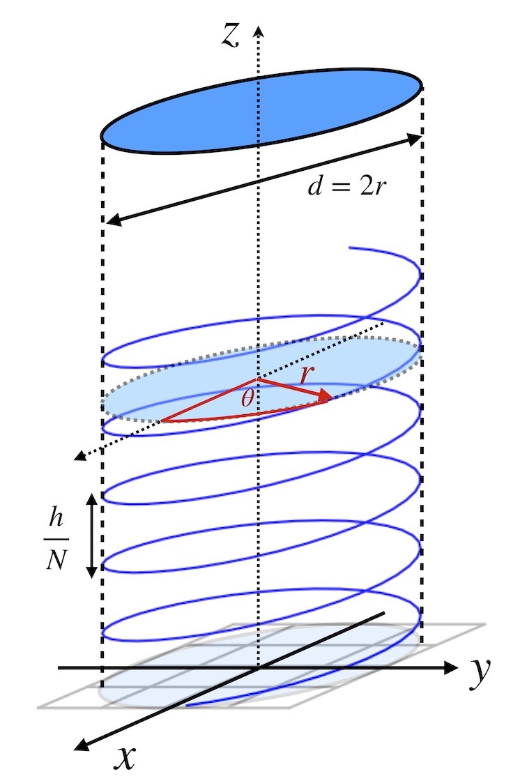
Then, in three-dimensional space, the coordinates \(x,y,z\) of the helix are parameterized by the angle \(\theta\) according to
\[\begin{eqnarray*} x &=& r\cos\theta, \\ y &=& r\sin\theta, \\ z &=& h\left(\frac{\theta}{360^\circ\cdot N}\right). \end{eqnarray*}\]
As \(\theta\) passes through each multiple of \(360^\circ\), then \(x\) and \(y\) come back to their original values but \(z\) increases by \(h/N\). After \(N\) revolutions the angle has advanced by a total of \(N\cdot 360^\circ\) and \(z\) has advanced a distance \(h\).
This set of equations may look a bit complicated, but imagine that we slice the surface of the cylinder along a line parallel to the axis, and then “un-roll” the cylindrical surface to form a flat plane. Here is the pattern that emerges:

The Surface of a Cylindrical Helix. A helical curve (blue) on a cylindrical surface that has been sliced parallel to the axis of the cylinder and un-rolled. The curve and its logarithmic scale begin at \(\theta = 0\), where the log scale starts at a value of 1. In our example, after 10 rotations the scale ends with a value of 10.
The numbers marked along the length of the curve on our helical slide rule follow a standard logarithmic scale, beginning at 1 and ending at 10. If \(d=2r\) is the diameter of the helix, then the total length along one of our \(N\) lines above can be calculated using the Pythagorean Theorem and is found to be \(\sqrt{(\pi d)^2 + (h/N)^2}\). Then, over a total of \(N\) spirals, we have a total length of \(N\) times this result, or
\[ L_{eq} = N\sqrt{(\pi d)^2 + (h/N)^2} = Nh\sqrt{(\pi d/h)^2 + (1/N)^2}. \]
If there is a large number of spirals and if the device is constructed such that its length \(h\) and its diameter \(d\) are of the approximate same scale, then the second term under the radical sign is much smaller than the first term, and the above expression reduces to \(L_{eq} \approx \pi d N\), as we approximated earlier. As an example, a one-inch diameter cylinder with a 30-turn helix will have a scale with an effective length of about 100 inches. This is ten times longer than the standard 10-inch slide rule, yet likely can still fit in a coat pocket.
With a scale at hand such as the one above, and rolling it into a cylinder, one now just needs to have a method for adding distances along the scale in order to perform multiplication calculations. Moving up and down the length of the major axis of the cylinder, there is a unique value of \(\theta\) for any value of \(z\) along the axis, which then corresponds to one unique value along the helical scale. So, one needs a device that can slide scales or indicators up and down along the axis, but that can also rotate the scale or rotate an indicator in order to read results along the curve. Various such methods exist, and depend heavily upon the design of the particular slide rule, but the fundamental principle is the same as for any other slide rule – adding distances along the logarithmic scales provides a multiplication calculation.
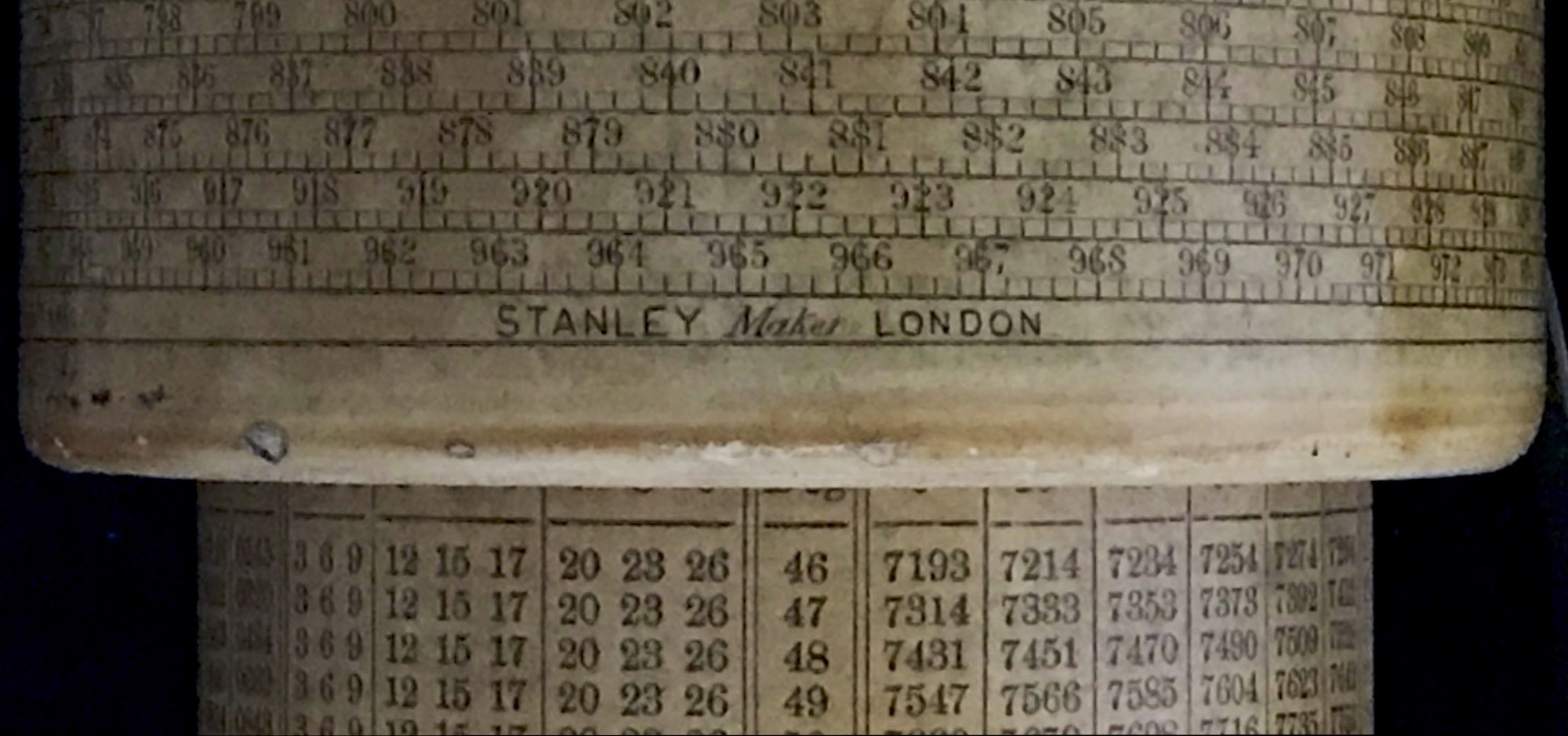
A variety of helical slide rules were manufactured by major companies, including McFarlane (Scotland), Stanley (London), Otis King (London), Browne (Melbourne) and others. Otis King was perhaps the most popular, and the Fuller Calculating Slide Rule by Stanley was likely the most accurate due to its large effective length. Both of these slide rules were in production for many decades, and I am fortunate to have examples of both in the Collection.
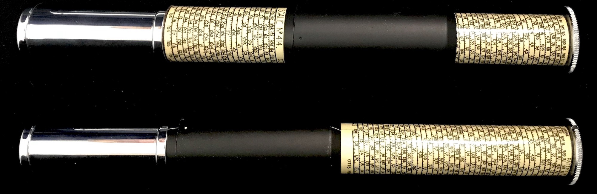
8.33.1 The Otis King
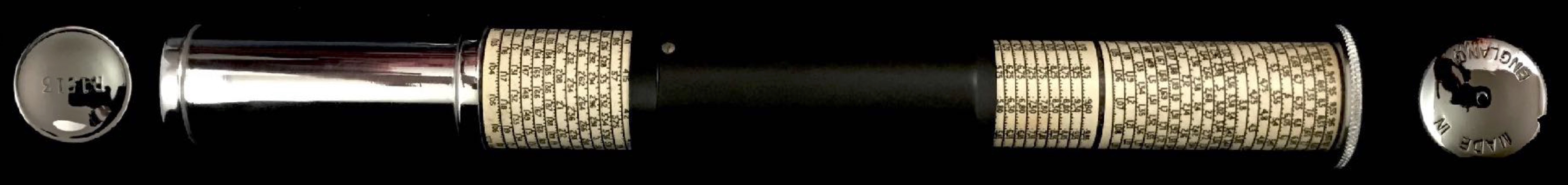
The Otis King’s Calculator, manufactured by Carbic Limited, London, was produced from 1921 until 1972. The patent for the device filed by Otis Carter Formby King in 1921 was accepted in August, 1922.145 The original models produced by Carbic (Models A-J) were made for business usage such as retail cash and wage calculations and are quite rare;146 but Models K and L were more generic and became popular for a wide variety of applications where greater accuracy was required in the calculations performed.
Each model consists of a thin base cylinder with a stainless steel handle from within which a rotatable cylinder of slightly smaller diameter can be extended by about 4 inches. This inner cylinder can be rotated using a “knob” at its end. When the inner cylinder is collapsed within the outer cylinder, the total length of the slide rule is about 6 in.
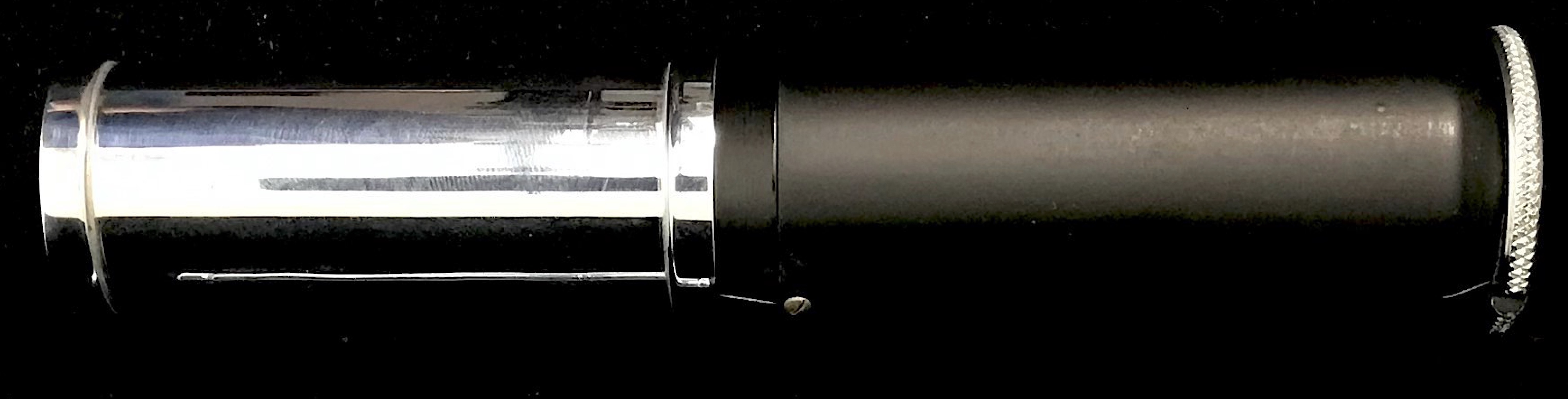
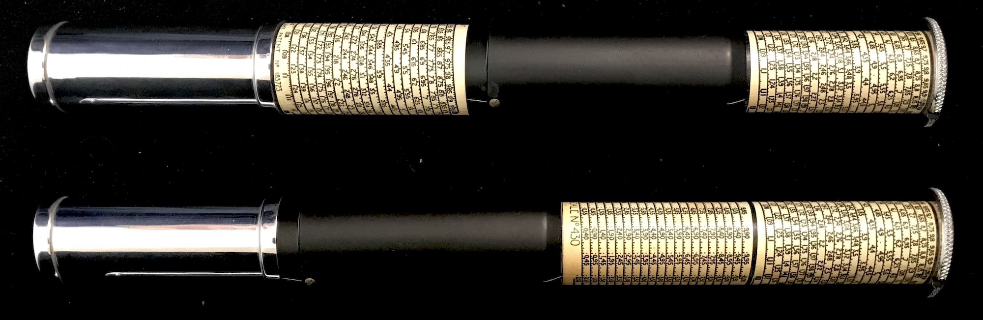
The base cylinder of the Model K in my possession has an outer diameter of about \(d\) = 1.05 in, and just above its handle begins a single-decade logarithmic helical scale. The total height of this scale on the cylinder is \(h\) = 2 in and contains \(N\) = 20 turns. Approximately 1.25 in above this single-decade scale is a two-decade scale, also of 20 turns per decade and with a total height of 4 in (2 in per decade).
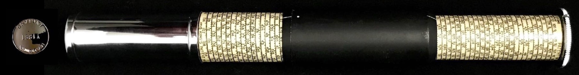
The Model L has the same outside dimensions when closed as the Model K, but the scales on the inside cylinders are slightly different. The base cylinder of the Model L is essentially the same one-decade helical logarithmic scale; however, the two-decade scale is replaced by a one-decade scale plus a linear scale along a helix of the same total length. The top and bottom log scales can be used for multiplications, while the linear scale provides the logarithms of the numbers on the log scales, thus allowing for calculations involving raising numbers to powers, etc.
Using the parameters provided above, we can compute the effective length of the logarithmic scales found on the Otis Kings:
\[ L_{eq} = 20\cdot\sqrt{ (\pi\cdot 1.05 ~{\rm in})^2 + (2 ~{\rm in}/ 20 )^2 } \approx 66 ~{\rm in} \]
The Otis King was popular for many years due to its fine construction and its ease of use, as well as its accuracy. To perform a multiplication (using the Model K, for instance),
- Fully extend the inner cylinder to expose the entire scale.
- Move the black cylinder down until its white dot at the bottom lines up with the first number, \(a\).
- Holding the knob at the top of the slide rule, and not moving the black cylinder, set the middle “1” on the helical scale to the white dot at the top of the black cylinder.
- Moving the black cylinder only, align its top white dot with the second number, \(b\).
+ Note: \(b\) will be accessible by either moving up or down, which is why we start by aligning on the “middle 1”.
- The product \(a\times b\) is then found at the white dot at the bottom of the black cylinder.
If this series of movements is studied for a moment one can see that we are simply adding distances along the axis of the slide rule – which are proportional to the logarithms of numbers – and hence performing the exact same calculation that are performed on a standard linear slide rule.
Further information and examples of calculations can be found in the Otis King instructions sheet.
For more information on the Otis King Calculators:
- Peter Hopp, “Otis-King Update”, Jour. Oughtred Soc., Vol4.2 (1995) p33.
- Peter Hopp, “Otis-King - Conclusions?”, Jour. Oughtred Soc., Vol5.2 (1996) p62.
- R.C. Blankenhorn, “The Otis King’s Patent Calculators - Catalogue Raisonne”, Jour. Oughtred Soc., Vol18.1 (2009) p49.
- Peter M. Hopp, Slide Rules – Their History, Models, and Makers, Astragal Press (1999) pp.112,150,
- Dick Lyon, Otis King’s Patent Calculator, http://www.svpal.org/~dickel/OK/OtisKing.html.
- International Slide Rule Museum, https://sliderulemuseum.com/British.htm.
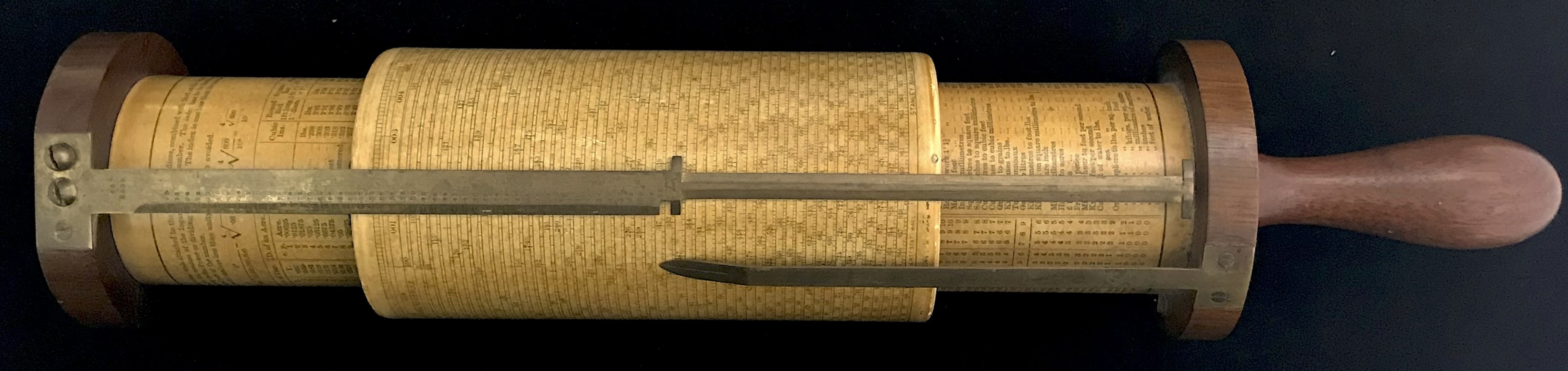
8.33.2 The Fuller Calculator
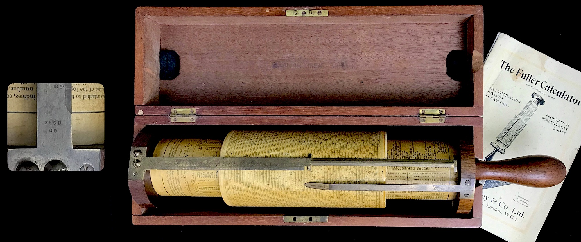
The Fuller Calculator is a helical slide rule that was manufactured from 1878 and various incarnations were sold for almost 100 years. There were two primary models (curiously named the Model 1 and the Model 2) and a few not-so-common models. Model 1 has a single helical scale for doing straightforward multiplication and division calculations. The Model 2 in addition has scales for sines and logarithms on its inner cylinder. A Model 3 “Fuller-Bakewell” also exists, which contains scales of \(\sin\theta\cos\theta\) and \(\cos^2\theta\) for use in stadia calculations, and there were special slide rules for coordinate transformations and for complex number multiplications. However, the Model 1 was the most popular and we are fortunate to have a Model 1 from 1909 in the Collection.
 |
 |
 |
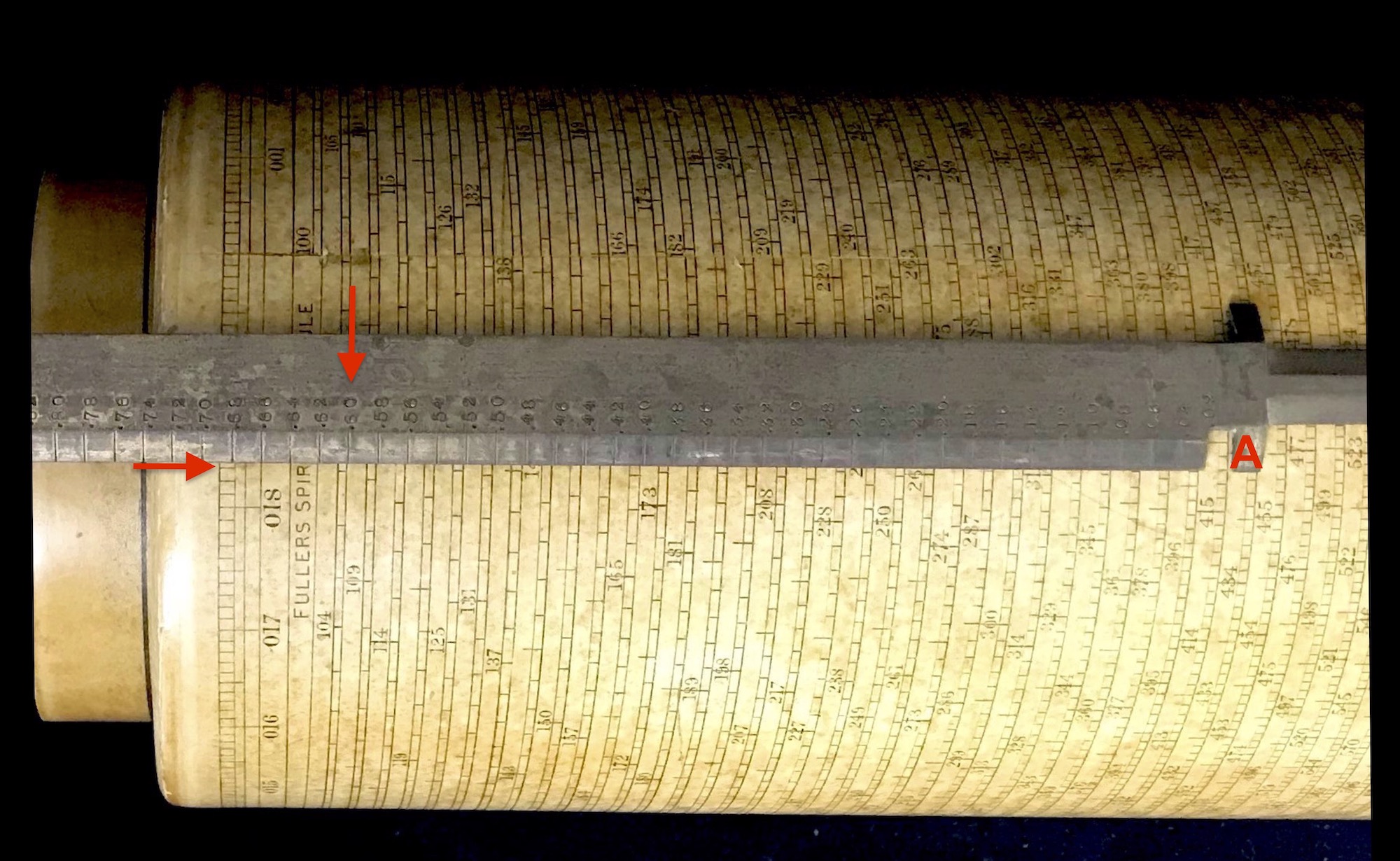
Our Fuller Model 1, which is labeled “Fuller’s Spiral Slide Rule”, was obtained from a bank in New Jersey, where they were “cleaning out the closet”. It has a frame made of mahogany, including its solid handle. Many of the more modern Fullers had a hole in the end of the handle which allowed for it to be placed into a rod to hold the slide rule up at an angle for the user. This early model has no such hole, and its early wooden box allows for the handle to protrude out the end of the box,147 while later models had boxes that surrounded the handle as well as the cylinder attached to it.
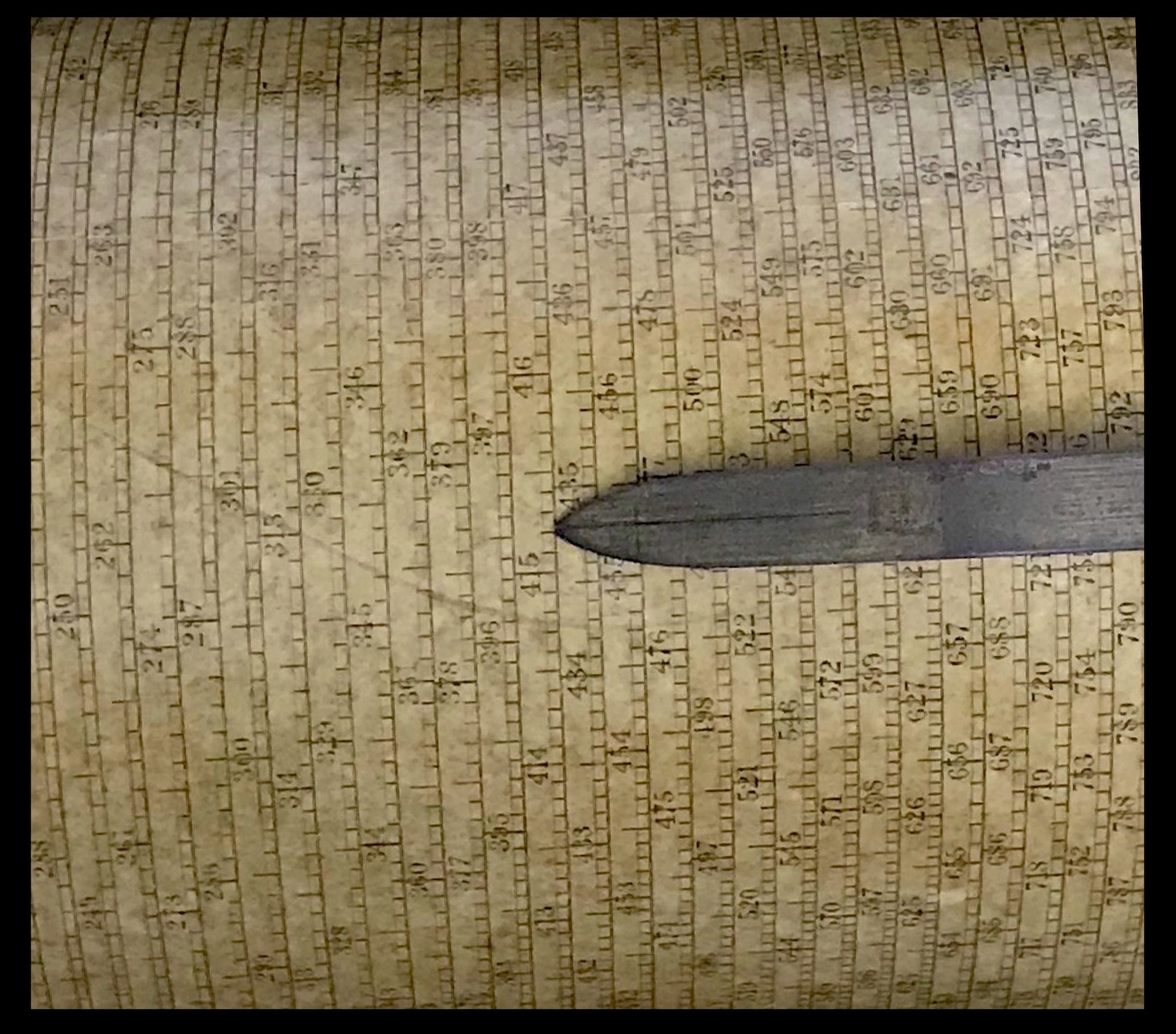
The main outer cylinder of the slide rule has a diameter of approximately \(d\) = 3.2 in and its scale has a total height of \(h\) = 5.5 in. The helix goes through a total of \(N\) = 50 rotations. Thus, the total length of the single-decade logarithmic scale on the slide rule is
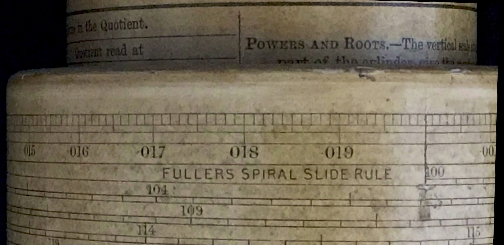
\[ L_{eq} = 50\cdot\sqrt{ (\pi\cdot 3.2~{\rm in})^2 + (5.5~{\rm in} / 50 )^2 } \approx 503~{\rm in} \] Since it is 50 times longer than the length of the standard 10-inch slide rule, the Fuller was able to compute answers to four significant figures without difficulty, and in many circumstances to five significant figures.
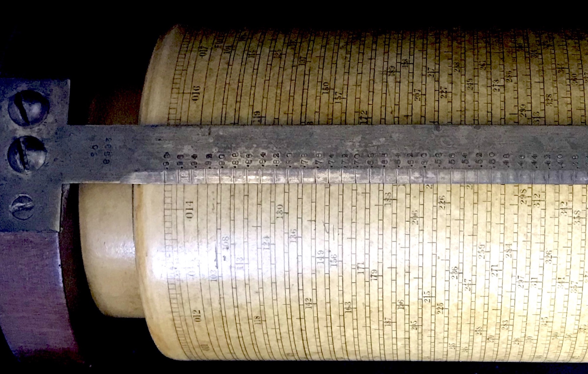
In addition to the 500-inch helical scale, there is a single-turn linear scale at the top of the outer cylinder which goes from 000 to 020, the “000” being aligned with the “1” on the helix. Since there are 50 turns in the helix, each turn around the cylinder increases the logarithm of a number by 0.02. So, by keeping track of what “turn” a number is on and by reading off the number on the circular “020” scale, the logarithm of any number on the helix can be found to approximately 4 significant figures. Counting the turn number is performed using a special scale along the major cursor of the slide rule, which runs from 0 to 100 in 0.02 gradation.
The Fuller uses two cursors to perform calculations. The longest cursor has two indicators A and B, one at the bottom end of the cursor (B) and one roughly mid-way down the cursor (A). This long cursor is attached to the top of the slide rule (the handle being at the bottom). This cursor can also be rotated independent of the base and of the main cylinder containing the logarithmic scale. Then, there is another, shorter cursor which is attached directly to the base of the slide rule. This cursor has a free “tip” which is referred to as indicator F (for “fixed”). If the scaled cylinder is moved to the bottom of the rule, then F can be aligned with 1 on the scale; if the cylinder is moved to the top of the rule, then F can be aligned with 10 on the scale.

To illustrate a basic multiplication calculation on the Fuller calculator, let’s take 173 times 24 to get 4152. We set the number 173 onto the fixed indicator, F. We then bring either the A or B indicators to either the 1 or 10 on the scale, whichever can be performed. (Like any slide rule, a number might go “off-scale” in one direction or the other.) In our case, we move the A to 1 (and the B makes it to 10). Then, we leave the indicators alone, and move the cylinder to line up 24 on the A or B indicators (A in our case).
The result will be found at the fixed indicator, F: 4152.
Again, if you carefully rexamine this series of movements you’ll be able to see that we are simply adding distances along the axis of the slide rule which are proportional to the logarithms of the numbers of interest.
To find the logarithm of a number using the Fuller, let’s take the log of our result above. Naturally, the log of 4152 is the same as 3 + the log of 4.152. Keeping that in mind, we slide the cylinder toward the top of the rule, and rotate it to align the number 4.152 with the A indicator. From our “020” scale, we see that the long brass cursor passes by the number 0183. We also note that the fractional number at the top of this cursor that lines up with the top line of the spiral scale is “0.60”. This tells us that the log of 4.152 = 0.60 (from the number of turns) + 0.0183 (from the fractional rotation) = 0.6182. Hence, the log of 4152 will be 3.6183. Let’s check by computer: \(\log(4152)\) = 3.618257.
Rather than going on with many other examples, the reader is referred to the well-written instructions that came with the Fuller Calculator.
Further information on the Fuller Calculators can be found at:
- Wayne Feely and Conrad Schure, “The Fuller Calculating Instrument”, Jour. Oughtred Soc. Vol 4.2 (1995) p33.
- Wayne Feely and Conrad Schure, “Update of Known Fuller and Thacher Rules”, Jour. Oughtred Soc. Vol 5.1 (1996) p25.
- Peter M. Hopp, Slide Rules – Their History, Models, and Makers, Astragal Press (1999) pp.113-114,221.
- Wikipedia, Fuller Calculator, https://en.wikipedia.org/wiki/Fuller_calculator.