8.32 Spring Calcs Eternal
Originally posted: 2022 Dec 23
Increases in industrial applications of springs in the 1930s and 1940s saw the development of slide rules that were used to calculate spring parameters, driven heavily no doubt by the production of defense equipment during the second world war. While the concept of a spring and its use had been around for quite some time, the need to be able to predict accurately the force or pressure needed to, for example, move a valve head or to monitor its setting, required careful design and calculation of spring dimensions and materials to be used. Imagine, for example, the need to set and to read back conditions of gauges and valves used to monitor and control a large airplane or ship long before the era of solid state electronics and digital equipment. The number of springs required and the variety of spring conditions could be incredibly large, and thus the repetition of spring design calculations could greatly be mitigated by a good slide rule design.
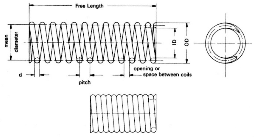
The basic equations being implemented in spring design are not too complicated, but do require a variety of numbers raised to various powers and multiplied or divided. A basic spring can be thought of as a wire, typically of circular cross section with diameter \(d\), coiled into a helical pattern, where the mean diameter of a coil is \(D\) and the number of coils created is \(N\). Two primary questions are, (a) what is the maximum safe load in pounds which the spring can support without breaking, and (b) by how much will the spring compress or expand due to a particular load?
The first question can be examined using the equation below, \[ P_{max} = \frac{\pi\;d^3 S}{8\;D} \] where \(P_{max}\) is the maximum safe load in pounds and \(S\) is the safe shearing stress, in units of pounds per square inch. The diameters \(d\) and \(D\) are in inches. (We are using pounds and inches here, as the slide rules were mostly created using this system of units.)
For the second question, if \(f\) (in inches) is the deflection or expansion of the spring for a load \(P\) (in pounds), then \[ f = \frac{8 N P D^3}{d^4 G} \] where \(G\) is called the torsional modulus of elasticity, in units of pounds per square inch. Note that both \(S\) and \(G\) are properties of the material being used to make the spring.
Our last equation can be re-formed in terms of what is called the rate of the spring, which gives the pounds of load per inch of deflection, \[ R = \frac{P}{f} = \frac{G}{8}\cdot\frac{d^4}{N \;D^3}. \]
8.32.1 The Sandish Scale
This last equation is one of the more common calculations found on spring slide rules. For example, an early home-made slide used for this basic calculation is shown in the figure below.
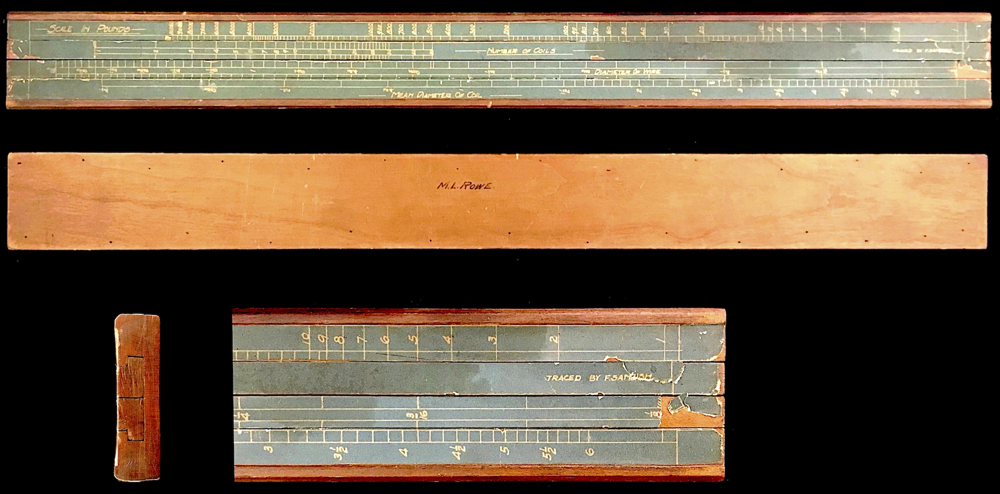
Made of several layers of plywood, this 20-inch-long single-sided slide rule has two slides, each with a single scale, and each with a slat that fits within a groove in the stock to keep the slide in place. The scale set, using our symbols in the equations above, is
R [ N ] [ d ] D
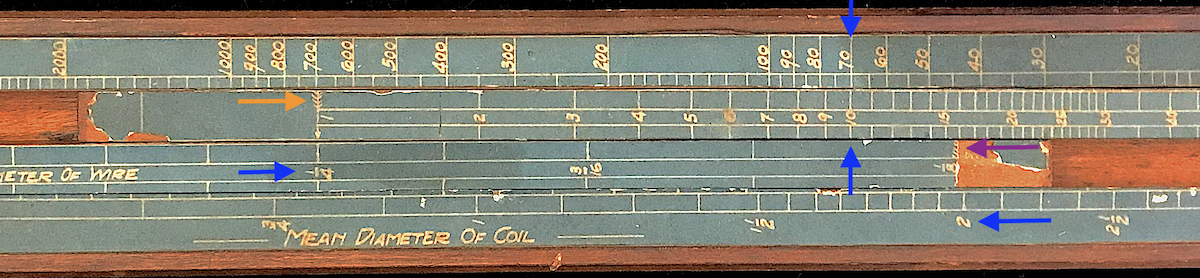
After a bit of fiddling around I was able to figure out how the slide rule was intended to be used. This was particularly difficult due to the fact that much of the paper scale was flaking off of the wood on the rule. But, near the “1/8” inch mark on the lower slide’s scale (d) the remainder of a special marking was discovered; this is where the calculation starts. (See purple arrow in figure below.) The user moves this “1/8” mark on d to line up with the value of D on the bottom scale that is to be used. Next, move the arrow on the left-hand side of the N scale (see orange arrow) to line up above the value of d to be used. Follow the N scale over to the number of coils in the spring, and above this value will be the spring’s rate on the R scale.
As a numerical example, the slide rule is set to perform the calculation for \(D\) = 2 in, \(d\) = 0.25 in, and \(N\) = 10, which is shown in the image below. The rate is found to be about 70 pounds per inch.
“Reverse engineering” this result, we can find out what value of \(G\) is being used in this calculation. Taking our rate equation above and solving for \(G\), we get \(G = 8RND^3/d^4.\) Taking the numbers from our example above, we find \(G\) = 11.5 million pounds per square inch is being used for this slide rule. This is a value found for carbon steels and alloys and is a common value used in spring calculations, with small adjustments sometimes made afterward for various other specific materials.
So, what is actually going on in this calculation using this slide rule? Taking a closer look we can measure the distances through a decade on each of the scales. For instance, the top scale R runs from 1 lb/in at the right, to 10,000 lb/in on the left. The fact that it runs from right to left makes this an “inverse” scale. The distance on the slide rule through a decade (1 to 10, or 100 to 1000, etc.) is measured to be about 4 inches on this scale. Next, running left to right, is the N scale, with a span from 1 to 50, where the distance from 1 to 10, or 5 to 50, is also 4 inches. However, the following scale on the second slide, d, has a range from about 1/8 of inch on the right to 1.75 inches on the left – another inverse scale – and its decade is actually 16 inches long. So as d advances by a decade, R will advance by 4 decades in the same direction on the slide rule. This tells us that \(R\) is varying like \(d^4\). Looking familiar? And finally, the bottom scale D has a range from 1/4 in to 6 in moving left to right, with a decade length of 12 inches – 3 times the decade length for R. And since its direction is inverse to that of R, then values on \(R\) scale like \(1/D^3\).
My guess is that the missing paper scale on the right end of d would have had a mark at 1/10 in, just to the right of the “1/8” mark. One can still see the “tail” of an arrow just to the right of the label for “1/8” on this slide. Aligning the 1/10 mark on the d scale to the desired value on the D scale below it, and finding the desired d value to its left is equivalent to multiplying \(D^3\) by the inverse of \(d^4\). Lining up the N scale’s left end at the value of \(d\) and moving to the right to find the value \(N\) is equivalent to a multiplication of the previous result by \(N\). The spring rate would be the inverse of this final number, and hence the upper scale runs right to left: \(R = G/8\cdot [(D^3/d^4)\cdot N]^{-1}\) Thus, the final answer would be above the value of \(N\), and located on the R scale, where the multiplication of \(G/8\) is built-in through the final placement of the R scale on the rule.
Perhaps not so intuitive, but it does work. Using this slide rule, a coil designer could, for example, assume a certain coil mean diameter and examine combinations of wire gauge and number of coils that would produce a necessary spring rate for the job at hand. The range of values of \(d\), \(D\), and \(R\) were likely determined by the types of items being constructed for this particular industry. A different company may have needed a different set of scale ranges for their production efforts.
8.32.2 The Baetzmann Slide Rule
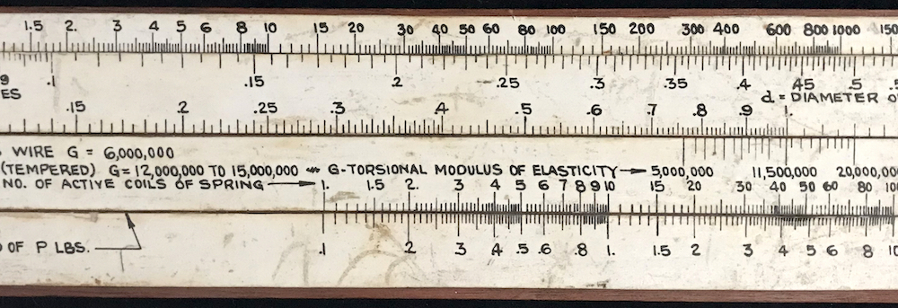
A slightly different, but perhaps more traditional approach was taken by Robert Baetzmann and his spring calculation slide rule. (See image below.) Another seemingly in-house produced slide rule, the Baetzmann rule is used to perform both of the two calculations described earlier, one on each of the two sides of the slide rule. The first equation for \(P_{max}\) can be evaluated by a single slide, as it involves only four parameters, if scales for two of the parameters are printed on the slide, and this is what is found on one side of the rule (bottom image). As the second equation for the rate \(R\) contains five parameters, the use of two slides similarly can perform this equation with room for one parameter left over. Baetzmann chose to divide up the rate into a load and a deflection, thus performing the entire calculation of six variables, and this is found on the other side of the slide rule (top image).
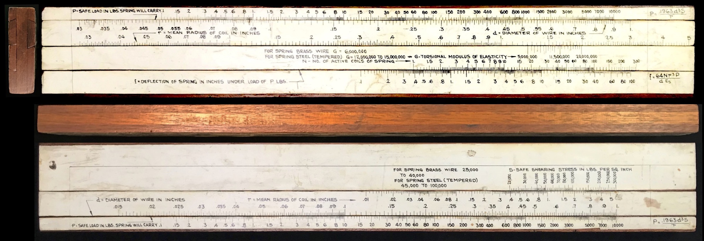
Note that on this slide rule, all the scales run left to right, but the ranges of the scales are similar to those found on the Sandish rule. Also note that Baetzmann chose to allow for various choices for the constants \(S\) and \(G\), and hence this slide rule can be used to evaluate springs for a variety of materials in a straightforward way, unlike in the Sandish rule. For more information about the Baetzmann slide rule see the vignette An Early Home-Made Spring Calculation Slide Rule.
The image below shows this slide rule set up to perform the same calculation as for the Sandish rule. Here, we set the value of N = 10 at the bottom of the bottom slide to line up with a deflection \(f\) of one inch on the bottom scale. We then set the 1 on the coil radius (D = 2) on the upper slide with the value of G = 11.5 Mlb/in on the lower slide. Next, we locate the wire diameter d = 0.25 on the top of the top slide, and finally read off the load on the upper scale: P = 70 lb (reminder: for a one inch deflection; hence, R = 70 lb/in).
8.32.3 Spring Rule Makers
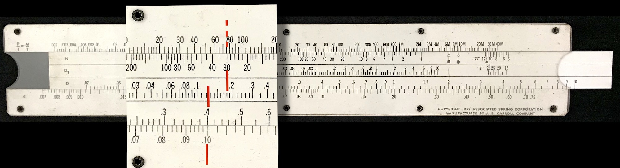
A nice article on the early production of spring calculation slide rules by the major slide rule manufacturers was written by Michael Konshak in 1997.144 Companies that produced springs for industry – most notably Associated Spring Corporation – produced slide charts for performing these calculations in the mid-1940s, but the major slide rule makers of the day did not produce their own models for spring calculations until about 1952.
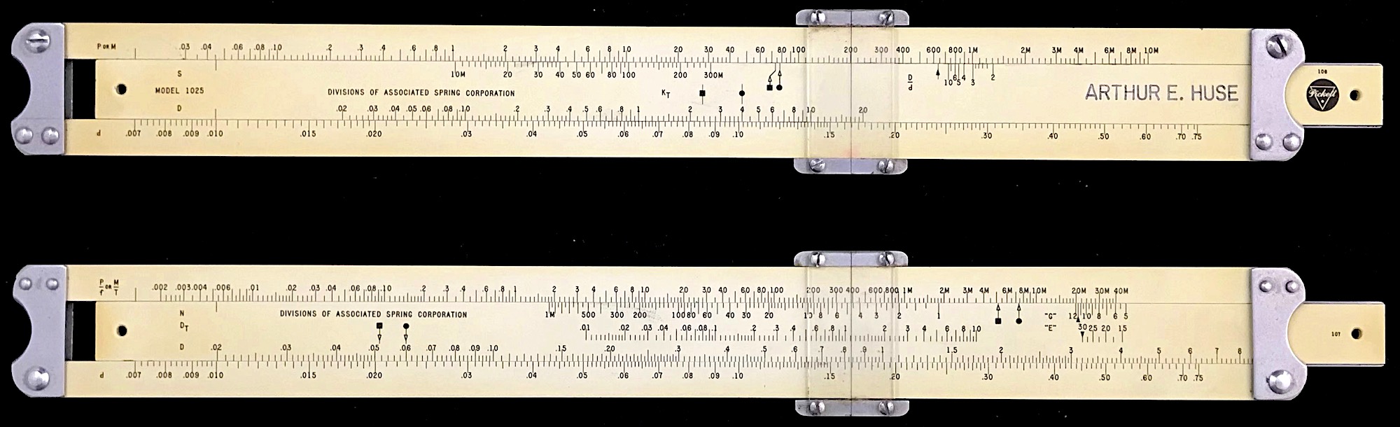
Pickett appears to be perhaps the earliest entry of the major slide rule producers to make spring slide rules, with their Model 1025. Our example is shown here:
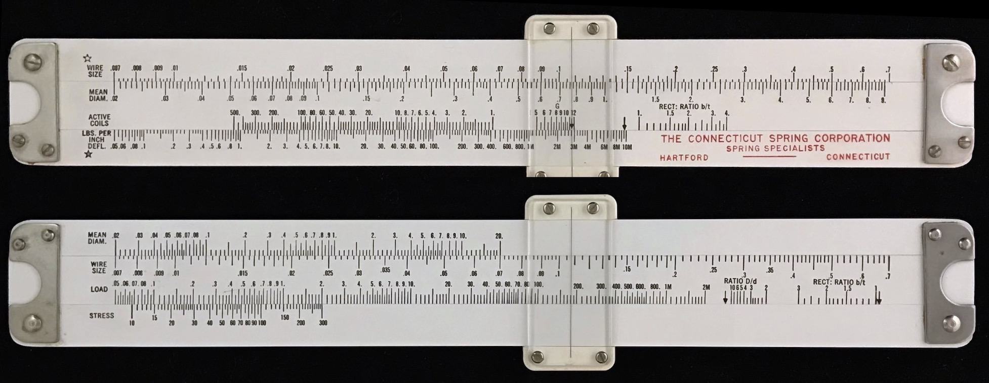
Other early examples include rules by J.B. Carroll and by Acu-Rule. These later examples all use the same scale set as was produced for the Pickett 1025. Below are images of the Carroll and Acu-Rule examples in the Collection.
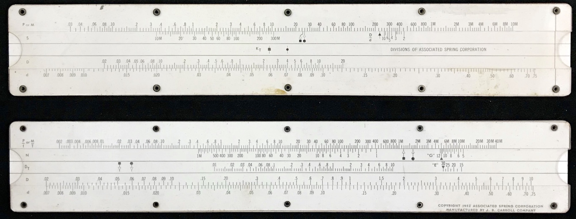
One can see that these mass-produced slide rules perform the same calculations as the Baetzmann rule, but through the use of a single slide. For these, variations in the constants \(S\) and \(G\) are performed, for example, by using the standard value of \(G\) = 11.5 Mlb/in, and then at the end of the calculation making an adjustment of the result by small additional movements of the slide using a second or third scale located on the bottom edge of the slide itself. While this keeps the slide rule design simpler in its components (one slide only), one could argue that having a layout like on the Baetzmann rule allows a designer to tweak independent parameters in the equation more readily. Dealer’s choice, I suppose.
Either way, being able to view many solutions all at once for one setting of the slide rule can be a big advantage to an engineer or designer. Compare this with using a hand calculator or a computer code/application. In the latter case, the user must input several variables and see what the answer is, and somehow keep track of it all as different values are typed in and computed.
Below is an image made of a computer code to compute the spring rate (variable Ponf) and the same calculation being performed on the J.B. Carroll slide rule. From the slide rule one can look and see immediately what the result would be of changing the number of coils; or, for instance, what wire diameter would be needed to get the same answer if the coil diameter were changed slightly. Doing this using the adjoining computer code would not be as straightforward (though codes can certainly be written to do the job).
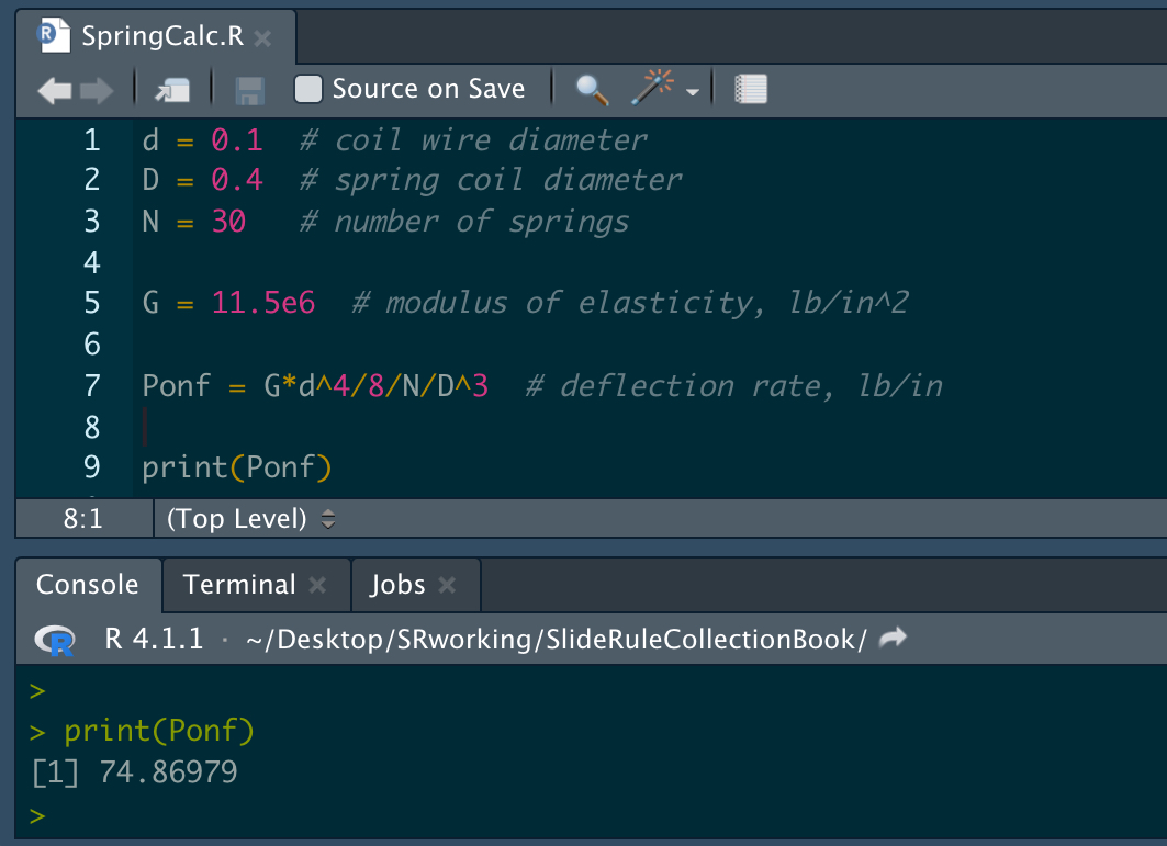
To illustrate a more modern approach, here is a quickly-written code to make a plot that attempts to convey the same process, by graphing \(d\) vs. \(D\) for various values of the product \(N\cdot R\), assuming a known value of \(G\). The dotted lines are for our example above where \(D\) = 2 in and \(d\) = 0.25 in; note that the intersection is at about N R = 700 (\(N\)= 10 and \(R\) = 70 lb/in, say).
G = 11.5e6   # lb/in2
NR = 1
d = function(D, NR){ (8/G*NR*D^3)^0.25 }
Ncrv = c(1:5)

plot(0,0,typ="n",xlim=c(0,10),   ylim=c(0,1),
                 xlab="D [in.]", ylab="d [in.]",
            main=paste("G =",G/1e6,"Mlb/in") )
i = 0
while(i<length(Ncrv)){
   i=i+1
   NR = (2*i-1)*100
   curve(d(x,NR),0.1,10,add=TRUE,lty=i,col=i)
}
legend(0,1,paste((2*Ncrv-1)*100),lty=Ncrv,col=Ncrv,title="N R [lb/in]")
abline(v=2,h=0.25,lty=3)
Which approach might be more desirable to a spring designer?
Side Note: About the Physics of Spring Rate and Hooke’s Law
Physics students generally learn about springs and forces (\(F\)) on masses (\(m\)) from the compression or extension (\(z\)) of a spring, according to Hooke’s Law,
\[ F = ma = m\frac{d^2z}{dt^2} = -k\;z, \]
when studying simple harmonic motion. The spring constant, \(k\), gives the value of the force required to move the mass through a displacement \(z\) from equilibrium, and so has units of force per distance.
Springs work through the torque produced from a uniform twist along the coiled wire when a force is applied at one end of the spring. This torque can be expressed in terms of a shear modulus, \(G\). We can first discuss what shear modulus is, and then use the result to look at how far a spring will stretch due to a load.
First, imagine a cylinder of material with radius \(r\), thickness \(dr\) and with length \(\ell\), being twisted due to an applied force tangent to the surface of the element as shown below.
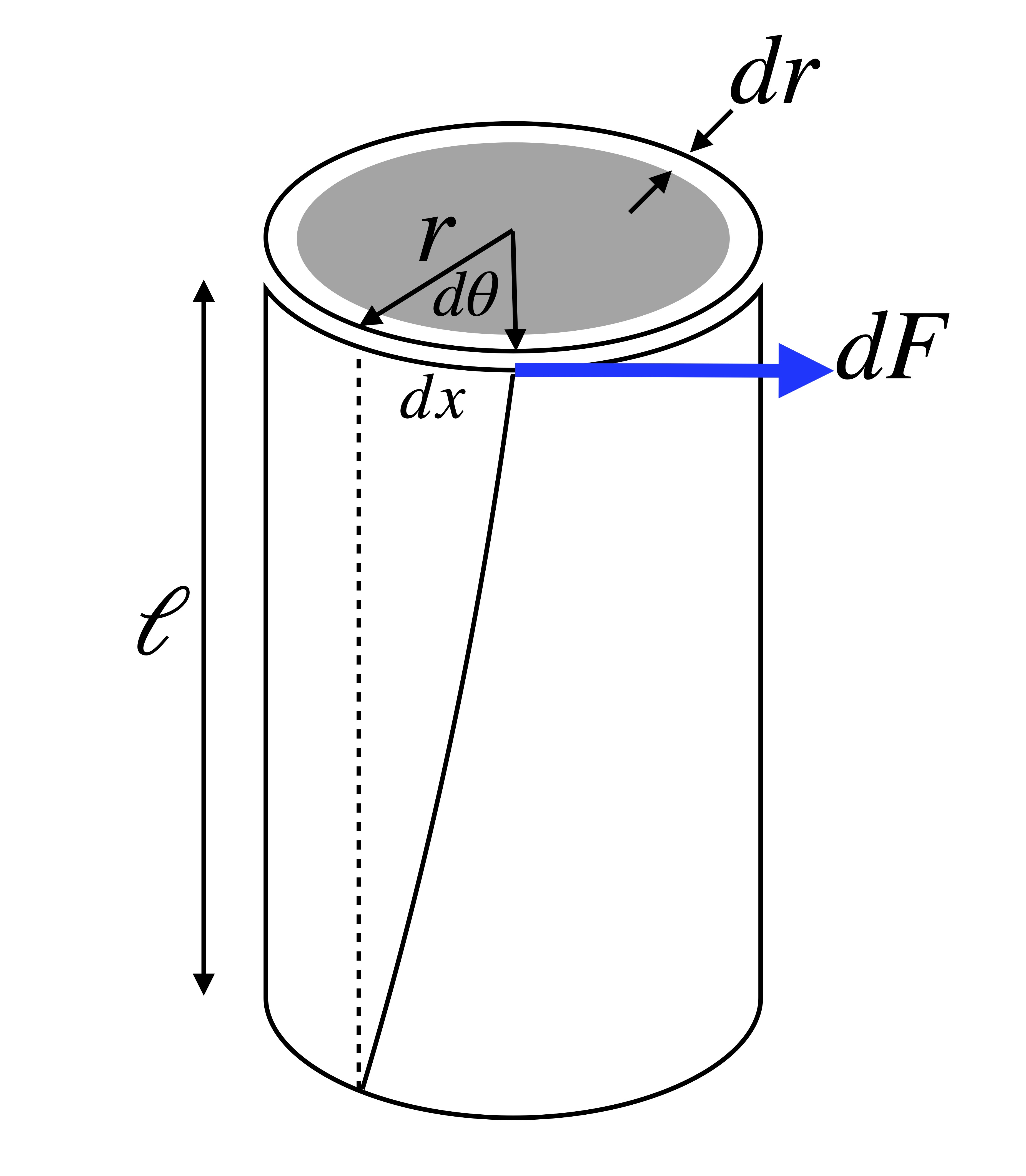
The torque generates a displacement \(dx\) over the length \(\ell\). In engineering terms, the shear stress in the material is the local transverse force through unit area, or
\[ {\rm stress} = \frac{dF}{2\pi r\;dr} \]
while the shear strain in the cylinder – the change in length due to stress – has the rate \(dx/\ell = rd\theta/\ell\) for our case. The shear modulus is defined in terms of the local torque as
\[ G = {\rm stress}/{\rm strain} = \frac{\ell\;dF}{2\pi r^2\;dr\;\theta} = \frac{\ell\cdot r\;dF}{2\pi r^3 dr\;\theta} = \frac{\ell\;d\tau}{2\pi r^3 dr\;\theta}, \]
or, in terms of \(G\), the local torque is
\[ d\tau = G\;\frac{2\pi\; r^3\;dr}{\ell} \theta. \]
Now find the total torque produced on all such cylinders within a wire of radius \(r\) by integrating over the total thickness of a solid cylinder. The total torque is
\[ \tau = \frac{G\pi \; r^4}{2\ell}\theta. \]
By definition, the torsion constant \(\kappa\) is torque per angle, and hence,
\[ \kappa = \frac{G\pi \; r^4}{2\ell}. \]
We will use this result in our next step.
Now imagine such a cylinder rolled into a spring, where the cylinder has diameter \(d = 2r\) and the resulting coil has mean diameter \(D=2R\). There are \(N\) full coils in the total length of the spring. (See our first figure above.)
Now, a force on the spring directed along the axis of the spring will stretch a local spring element through an angle \(d\alpha\) stretching the spring a distance \(dz\), where \(dz = R\;d\alpha\) as shown below.
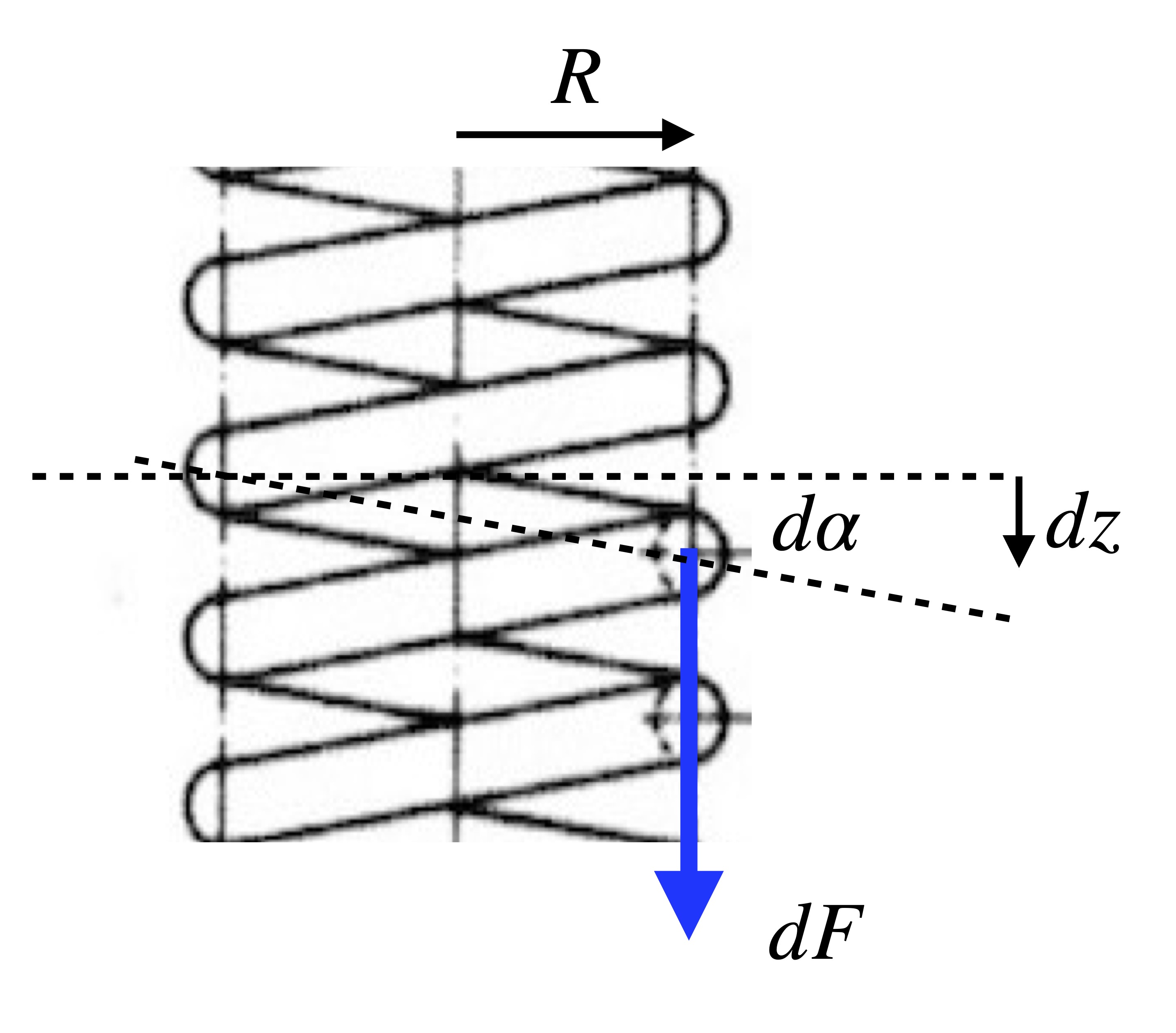
The angle \(\alpha\) will be small for the forces useful in the spring application. So, the total displacement of the spring when a full force is applied will be the integral of the above
\[ z = R\alpha. \]
Lastly, we calculate the energy stored in the spring in two different ways and equate. Firstly, in terms of the spring constant \(k\), we integrate Hooke’s Law to get \(E = \frac{1}{2}k z^2\). But, in terms of torques and angles, we can also write the stored energy as \(E = \frac{1}{2}\kappa \alpha^2\). Recalling that \(\alpha = z/R\), we see that \(k z^2 = \kappa (z/R)^2\), or, the spring constant is given by
\[ k = \kappa/R^2 = \frac{G\pi \; r^4}{2\ell R^2}. \]
And, since the total length of the wire in \(N\) coils is approximately \(\ell = 2\pi R\cdot N\), then
\[ k = \frac{G \; r^4}{4 R^3 N} = \frac{G}{8}\cdot\frac{d^4}{D^3N}. \]
Also, since \(k\) is the force required per displacement of the spring, this spring constant is simply the rate of the spring as described in the above text.
Michael Konshak, “The Spring Design Slide Rule Calculator”, Jour. Oughtred Soc., v15.1, p28 (2006).↩︎