8.38 How Do You Byoutou?

Over many years a complete listing of Hemmi manufactured slide rules was developed by Paul Ross, and compiled on his “Slide Rule Trading Company” (SRTC) web site. Actually, he created two lists – one of Hemmi slide rules with model numbers, and a second list of Hemmi slide rules that did not have a model number. Today these lists can be found at the web site of the International Slide Rule Museum (ISRM). Recently I came across a Hemmi with no model number. I was intrigued by the fact that it had a large number of scales of various lengths, most all of which were labeled as (1), (2), (3), and so forth, as opposed to any standard labels. I readily found the slide rule in Paul’s second list, where he referred to it as the “Byoutou” model of 1944. Apparently “byou tou” comes from the two characters that were found on the box containing the slide rule in Paul’s possession. I will continue to refer to this model as the Byoutou, but acknowledge that there may exist a more appropriate name to use.

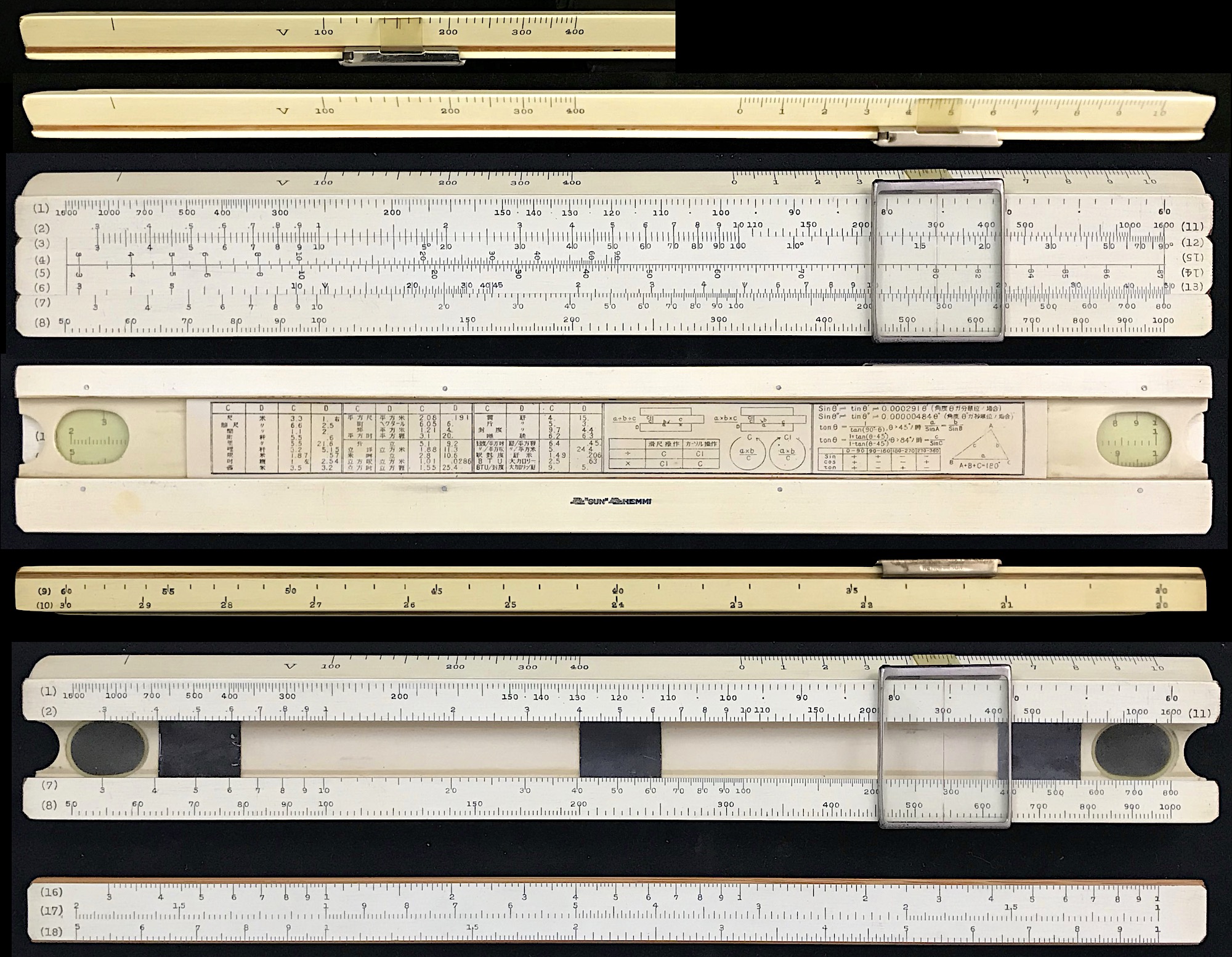
The Byoutou is a simplex slide rule about the same size and stock as a Hemmi Model 50W. However there is no model number on the rule and it has no date stamp. The scales are labeled on the left and right sides of the rule, and on the back of the slide, with numbers (1), (2), … (18). Two scales (14 and 15) are simply re-labeled scales (4 and 5) but with the labels upside down, indicating that the slide presumably is to be turned upside down (reciprocal scales) when using them. There are also two scales on the top edge of the rule, one labeled V and the other – a linear scale with cm spacing – unlabeled. Thus, there are 18 individual scales in all, 15 on the front and edges of the rule and 3 on the back side of the slide.

A cursory look at several standard collector’s sites only revealed to me two other examples of the Byoutou – the one owned by Paul Ross and discussed on his site, and another one on display at the ISRM web site. ISRM curator, Michael Konshak, reproduces much of the material regarding this rule from Ross’ web site on the ISRM site, but also discusses how his item was given to him by a former employer. At the time of this writing I did find one other example of this slide rule for sale online (without a cursor). Ross claims that, “These rules are relatively common but cursor is usually missing.” It now also can be found on Following the Rules (with cursor). If anyone knows of other examples that can shed light on this topic, please contact me.

The Hemmi Byoutou Slide Rule of 1944.

8.38.1 Byoutou Application

Inspection of the Byoutou reveals a variety of scales of common functions. There are logarithmic scales in which a decade (from 1 to 10 say) is 10 cm in length, and others with a 20 cm decade length. Most of these have the scale extended, typically on the left end, though a couple of the log scales cover only a partial decade. Other scales are clearly standard trigonometric scales. Some of these are labeled as “degrees” and extend to 45, or 90. Others are scales that have no unit given, but as they end at numbers such as 800 or 1600 they could be interpreted as having units of “mils”, where 1600 mils = 90 degrees. Most of these scales can be readily identified as sine, tangent, and even a “cosine times sine” scale. A few of the scales on the rule are inverted, running right to left. And some of the scales share a line across the slide rule. For instance, Scale (2) is a log scale that runs from 0.3 to 1 to 10, and ends just over midway on the rule; at this point a new scale – (11) – begins and runs from values of 110 to 1600. Scale (11) is a sine scale where the angles are in units of mils.

Two special scales can be found on the upper edge of the Byoutou. The first is labeled V and runs from 100 to 400. This is a partial logarithmic scale, where a full decade would have a length of 10 cm. A linear scale is to the right of the V scale. This scale, unlabeled, runs from 0 to 10 and is exactly 10 cm long, so it can be used for measurements along the upper edge. But this scale can also be used as an L scale in conjunction with one of the 10-cm logarithmic scales. Note that the cursor extends over the top edge so as to provide readings on the V and “L” scales that are aligned with the main scales on the body and slide. The zero of this “L” scale is aligned with the ends of Scales (2) and (3), which are also the beginnings of Scales (11) and (12). In addition, the 100 on the V scale is aligned with the 1 on Scale (2) and the 10s on Scales (3) and (7).

The large variety of trigonometric scales, and with mils being used, is strongly suggestive of a military application for this slide rule. In fact, from the references noted above, a naval application is suggested. Again from Ross, with information provided by Atsushi Tomozawa:

“Development History of the Slide Rule by Jihei Miyazaki states that the Byoutou rule was introduced in 1944 but does not mention what function the rule served. Another book, History of the Slide Rule, written for the Royal Navy Military Schools in 1944, explains how to use the rule to calculate a correction angle for firing at moving ships; the corrected angle is called corrected byoutou.”

I have not been able to track down copies of these books to review; any help in that matter would be strongly appreciated. The references to military schools might be suggesting that this rule could have been used for training purposes.

It has been pointed out to me¹³⁷ that the Japanese characters – 苗頭 – pronounced “Byoh toh” – have the meaning, “Deflection (gunnery).” In the context of ballistics, “deflection” is the art of aiming a projectile ahead of a moving target in order for them to meet at a point.

Meanwhile, from a slide rule forum on the groups.io site, I was guided toward a blog site from Japan where I found a short discussion of this very rule. The blogger did not know how to actually use the scales of the slide rule, but did “verify” that it was likely used to train junior officers in the basics of ballistics. According to Jeikan,¹³⁸ as translated from Japanese through Google Translate,

Initially, the task of calculating the seedheads [leading angles] of artillery and issuing instructions was solely the job of specially trained officers, who had learned ballistics from the theory of motion physics and mechanics, and who probably had little more than an ordinary slide rule and graph paper. It would have been possible to calculate the basics, but “As the war of attrition progressed, the absolute number of junior officers became insufficient, and it was necessary to select those who qualified for the first rank from among the conscripted active-duty soldiers, without providing them with in-depth training in theory, etc.” In order to teach the children [younger officers] only how to operate the special slide rule on a case-by-case basis and have them calculate the seedlings [leading angles], it was necessary to create a new simple slide rule that avoids difficult symbols and uses all numbers in parentheses. I think this was the reason why two types of slide rules for artillery were created, the old and the new. There should also be a textbook accompanying this slide rule, but I have not seen it yet.

The text above in brackets is my own interpretation of the generated translation.

So for now, let’s continue studying the scales on the rule more closely to see what we are truly dealing with. Then, we will look at possible applications in the area of ballistics.

8.38.2 Some Standard Scales

Because none of the scales have actual identifying labels, and since some are short and some are long, and since some extend beyond any standard range of values, I created images of scales and overlaid them on images of the slide rule to verify the functions being represented. A few examples of the scales that I used are reproduced below:

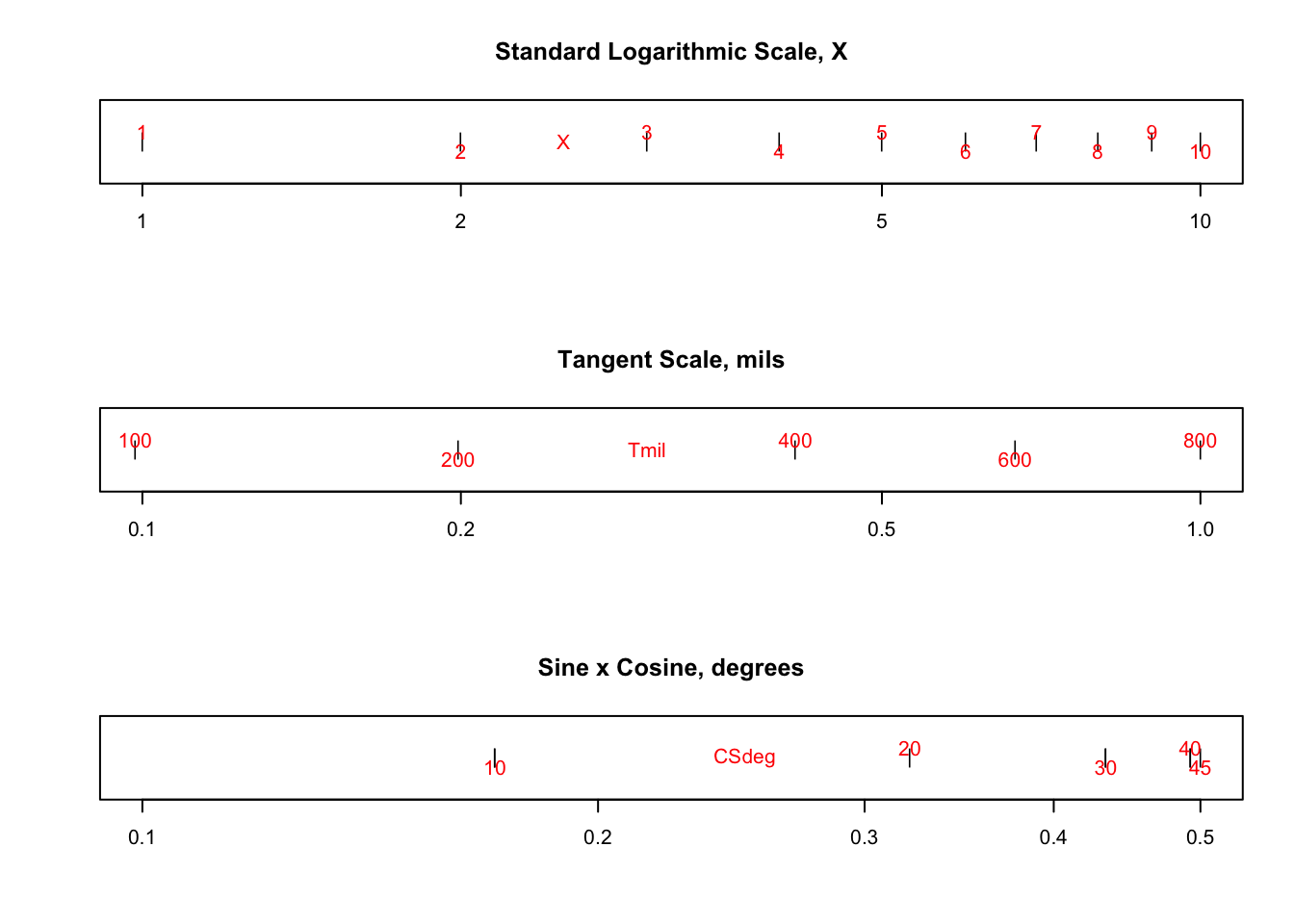
From this process I was able to verify the following scales on the Byoutou slide rule:

Location	Scale	Range (L-to-R)	Length (cm)	“Type”	Notes
top edge	V	100 - 400	6	A	partial log scale; decade = 10 cm
	“L”	0 - 10	10	cm	10-cm linear scale
stock top/left	(1)	1600 - 60	26.1	?	?? (presumed mils)
	(2)	0.3 - 10	15.3	A	extended log scale; decade = 10 cm
slide/left	(3)	3 - 100	15.3	B	extended log scale; decade = 10 cm
	(4)	3 - 90	16.1	S	Sin scale, deg., assoc. w/ (2)
	(5)	3 - 87	26.1	T	Tan scale, deg., assoc. w/ (2)
	(6)	3 - 45	10.1	CS	CosSin scale, deg., assoc. w/ (2)
stock bottom/left	(7)	3 - 800	25.4	T	Tan scale, mils, assoc. w/ (2)
	(8)	50 - 1000	26.1	D	extended log scale; decade = 20 cm
bottom edge	(9)	60 - 30	26.1	?	?? (continuation of (1)?)
	(10)	30 - 20	26.1	?	?? (continuation of (9)?)
stock top/right	(11)	110 - 1600	10	S	Sin scale, mils, assoc. w/ (2)
slide/right	(12)	10 - 90	10	?	?? (presumed degs.)
	(13)	2 - 50	14	B	folded log scale; decade = 10 cm
	(14)	87 - 3	26.1	TI	Scale (5), reversed
	(15)	90 - 3	16.1	SI	Scale (4), reversed
slide/back	(16)	3 - 1000	25.3	B	extended log scale; decade = 10 cm
	(17)	21 - 1	26.1	CI	extended reversed log scale; decade = 20 cm
	(18)	5 - 100	16.1	C	extended log scale; decade = 20 cm

The “Type” column indicates a more standard labeling of each scale, but is really only suggestive. For example, the A/B scales are logarithmic scales that have half the decade length of the D/C scales, and are found on the stock/slide of the rule. Also, all trig scales listed above are associated with an A/B scale rather than a C/D scale. Importantly, however, the trig scales (4), (5), and (6) on the slide are offset from the standard logarithmic scales when the slide is centered.

8.38.3 Non-Standard Scales

As can be seen in the table above, four scales are not described by standard log scales, trig functions, log-log, and so on. Below we go into investigations into these scales, namely (1), (9), (10), and (12).

8.38.3.1 Scale (12)

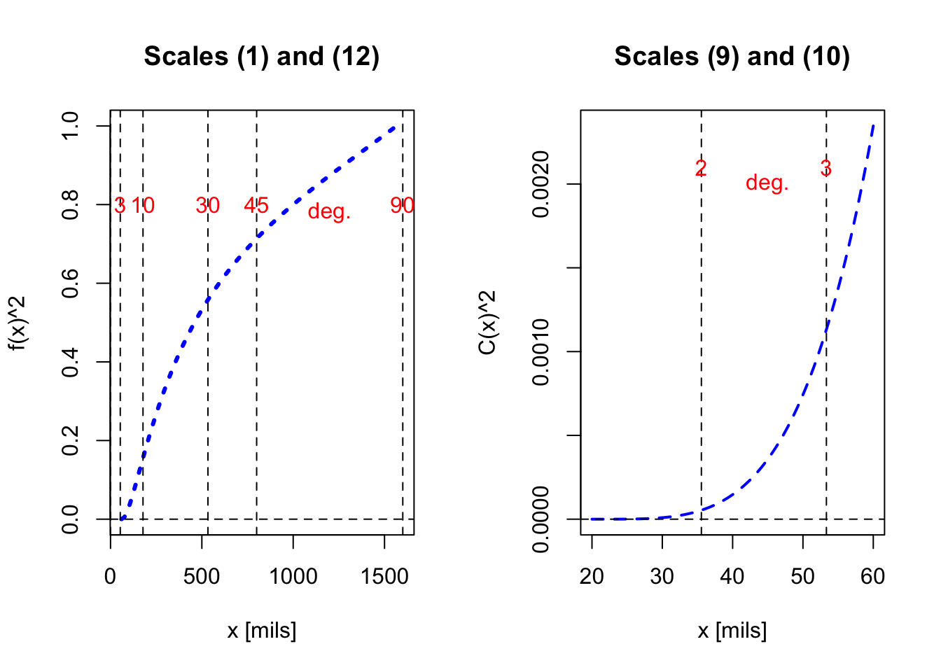
Scale (12) appears to represent a function whose argument is in degrees (from about 10 to 90). It ends at the right-hand side of the slide, so let’s assume this function has a value of 1 for an angle of 90 degrees. If we line up the right-hand side of a 10-cm decade logarithmic scale (using Scale (2), say) against 90 on the (12) scale we can read off values of our function, call it \(f_{10}\), against values of degrees. Of course lining up 90 degrees with a value of 1 is only one possibility. Besides the possibility of an overall scaling factor, it is quite possible that the angle values associated with this scale could be “inverted”. Or, there could be half-angles or double-angles involved, etc. However, the placement of (12) directly underneath a “mils” scale that goes to 1600, both of which are located directly underneath the “L” scale going from 0 to 10, suggests to me that a left-to-right reading of the function is most likely appropriate and that it is associated with the 10-cm-decade log scale. In addition, it might be that a result of 1 should indeed be interpreted as a result of 10, or some other factor. In any event, we continue on. Our effort produces the following plot:

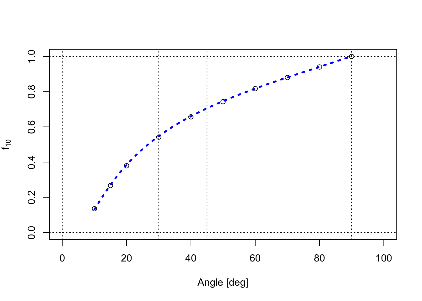
The blue dotted curve shown, arrived at by (a great deal of) simple trial and error, is

\[ f_{10}(x) = \left[0.983-\frac{0.175}{\tan(x+5.73^\circ)}\right]^2 \]

for \(x\) in degrees. At this point it is only one example of a function that mimics the points on the curve, using standard trigonometric functions. Though it does bear some interesting features, any of the three constants in the above could easily be influenced by my ability to line up the slide and read numbers from the scales.

So, we still don’t know at this stage what this function is for, or even if we are interpreting things correctly. But for now let’s proceed to investigate the remaining three scales.

8.38.3.2 Scale (1)

Scale (1) is a reversed scale and extends nearly the full length of the rule, which might imply that the values of the function are to be read from a 20-cm-decade log scale [(8), (17), or (18)]. Its value on the left end is 1600, while at the right end it is 60.

At this point I must stop to admit that it took me awhile to discover the following: If one removes and flips the slide, and lines up the 90 degree mark on the reversed-(12) with the 1600 mils mark on Scale (1), one can easily verify that the two scales can be used to convert mils to degrees and vice versa. For example, lining up the 90 deg mark on (12) with 1600 mils on (1) then the 45 deg mark lines up with the 800 mils mark, the 30 deg mark lines up with 533 mils (=1600/3), and so on. This tells us that Scale (1) actually represents the same function as Scale (12), and is to be read from the same log scale, which we previously assumed to be a 10-cm-decade scale. If, in fact, the values of our function are to be read from a 20-cm-decade scale, it would still be true that (1) and (12) are essentially the same scales, in mils and degrees, respectively. Also, our “trial” function – which is the square of a separate function – perhaps gives us a clue as to which log scale we should be using to read off values. For this reason, we next will use a 20-cm-decade.

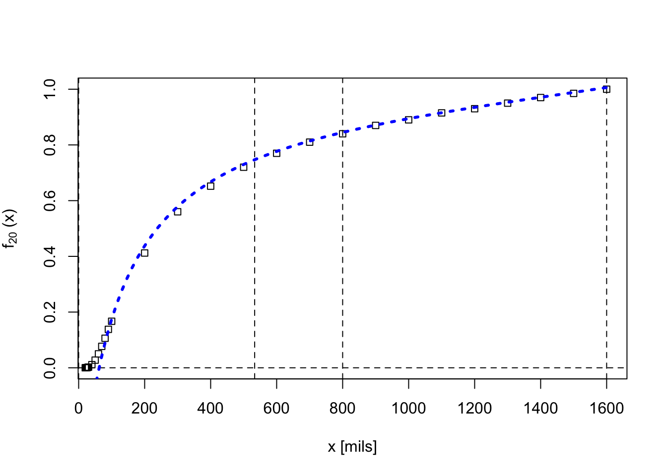
On the back of the slide, Scale (18) is an extended 20-cm-decade logarithmic scale from 0.5 to 10. I used this scale to plot out values of the function on Scale (1). Below is the result:

In the plot above, the black circles are values taken using Scale (1) while the red triangles are the values taken using Scale (12), converted to mils. All values of the function are read from proper re-positioning of Scale (18). The square root of our previous “trial” function is plotted in blue, though parameters were adjusted slightly to get better alignment:

\[ f_{20}(x) = 0.98-\frac{0.178}{\tan(x+120~{\rm mils})}. \]

To summarize, Scales (1) and (12) are indicative of a function \(f\) that, if read off of a 20-cm-decade log scale, goes something like

\[ f(x) \sim 1 - \frac{k}{\tan x} \] with perhaps some offsets involved.

8.38.3.3 Scales (9) and (10)

Scales (9) and (10) on the bottom edge of the slide rule are also reversed scales and also extend the full length. Note that while (1) goes from 1600 to 60 left-to-right, (9) goes from 60 on the left to 30 on the right, and (10) goes from 30 on the left to 20 on the right. So, it could be that (10), (9), and (1) represent a single scale set, split into three segments. Note that the edge scales (9) and (10) do not have any subdivisions. In fact, the cursor does not extend to these scales and hence one expects that values of the elusive function(s) we are seeking here are not very significant to the intended problem at the fractional-mil level.¹³⁹

If we attempt to combine Scales (1), (9), and (10) into one continuous function, using a 20-cm-decade scale to read values, we get the following, where the blue curve is our \(f_{20}\) curve given above:

It seems possible to me that Scales (9) and (10) might be used in lieu of Scale (1) in order to provide a more accurate result for very small angles, taking into account other properties of a particular gun system. The close-up below is for only the two scales found on the lower edge of the slide rule. The numbers on Scales (9) and (10) are interpreted to be mils, and the function values are taken from a 20-cm log scale.

The two curves above are fit by eye, using a “quadratic” function. Actually, the blue curve is \(C_{20} = ((x-20)/180)^2\), while the red curve is, \(C_{20} = 64[1-\cos(x-20)]\). I also note that to obtain each curve I assumed that the value at 60 mils on Scale (9) is the same as the value at 60 mils on Scale (1), and that the value at 30 mils on Scale (9) is the same as the value at 30 mils on Scale (10), which actually may not be the slide rule designers’ intention.

Reading and plotting the (9) and (10) scales independently, taking values from the 20-cm-decade scale, we find:

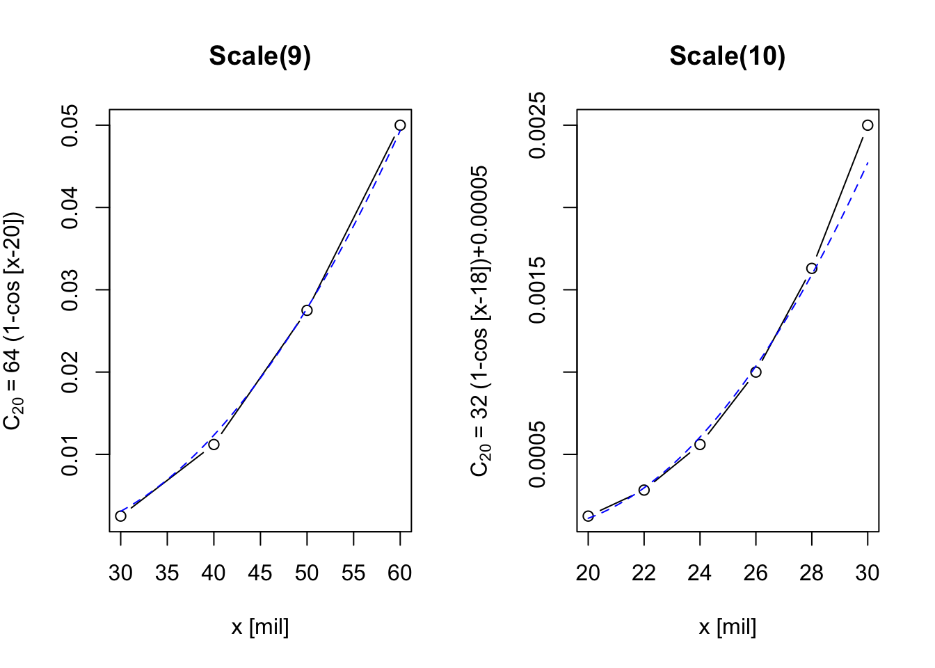
where the blue dashed curves are the functions \(C_{20}(x)\) as shown in the vertical axis labels.

Repeating with values being associated with 10-cm log scales:

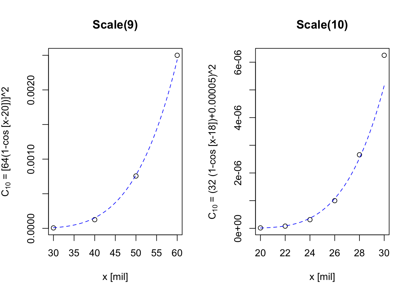
One might imagine using (10) from 20 to 28 mils, (9) from 30 to 59 mils, and (1) from 60 to 1600 mils.

With general functional forms in mind for the special scales on the slide rule, a final check can be made by generating images of the scales and overlaying them on images of the slide rule. Since the other trig scales are tied to the 10-cm log scales, we will assume them to be used with an \(f_{10}\) scale. Below is an image of the Byoutou slide rule showing Scale (12). Superimposed is a scale made from our “trial” function, where further tweaks have been made to two values in order to produce a better fit to the scales on the rule:

\[ f_{10} = f_{20}^2 = \left[ 0.983 - \frac{0.175 }{ \tan(x+5.73^\circ)}\right]^2. \]

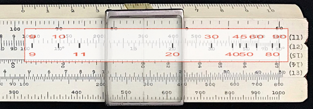
Taking our self-generated scale, flipping it, and aligning it over Scale (1), we see that the “degree” values align fairly well with their corresponding “mils” values.

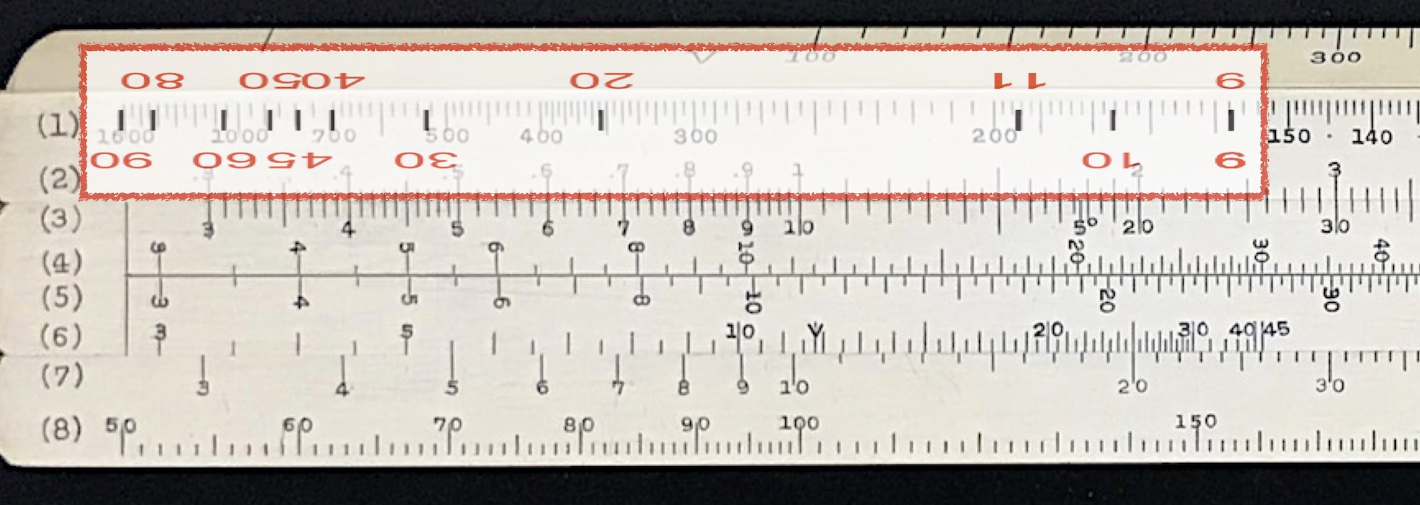
Performing a similar analysis for Scale (9) shows that it conforms well to the function \(C = 64[1-\cos(x-20)].\) Scale (10) is close, however it does not conform nearly as well to its previous functional form when overlaid on the slide rule.

Regarding the special scales of the Byoutou, here are my conclusions thus far, subject to change given the uncertainties in our approach:

• Scales (1) and (12) are describing the same function, with Scale (1) in mils being the inverse of Scale (12) in degrees.
  • limits for Scale (1): from 60 mils / 3.4 deg to 1600 mils / 90 deg
  • limits for Scale (12): from 178 mils / 10 deg to 1600 mils / 90 deg
  • Note: As both 10-cm and 20-cm log scales are found on the rule, one can think of any function being \(Y(x)\) on the 20-cm scale, and \(Y^2(x)\) on the 10-cm scale.
    
• Scales (9) and (10) could be independent of Scale (1), but are likely extensions of (1) to be used for the same purpose, only for very small angles.
  
• With the above assumptions,
  • Characteristically, Scales (1) and (12) are well described by a function of the form \(f(x) = f_{20} = \sqrt{f_{10}} \sim 1-k/\tan(x)\) using a 20-cm scale.
    
  • Scales (9) and (10) are suggestive of functions of the form \(C(x) = C_{20} = \sqrt{C_{10}} \sim 1-\cos(x) \sim x^2\) for small \(x\) also using a 20-cm scale.
    • Scale (9) fits well to a \(C \sim 1-\cos x\) function over the range 30 to 60 mils
      
    • Scale (10), not as much
• If we assume that our special functions have values of 1 at 90 degrees (1600 mils), and assume that they are to be used with the other trig functions on the rule which are connected to 10-cm-decade log scales, then these special functions might look something like this:

So what do we do with all of this? Taking a hint from our previous source, Paul Ross, let us next look at what we can learn by studying the mathematics of external ballistics.

---

8.38.4 Ballistics Basics

The term internal ballistics refers to the study of the motion of projectiles being fired from a gun or cannon while inside the device. External ballistics is the study of what happens to the projectile – its trajectory – once it leaves the device. As with any introductory physics problem, we begin by taking a standard “Freshman” approach and ignore details such as friction, air resistance, curvature of the earth, Coriolis force, and so on. It is quite likely that the problems being dealt with here cannot ignore all of these effects, and so we will next add in the the most important effect, air resistance.

Ballistic Basics – Sketch of the Problem.

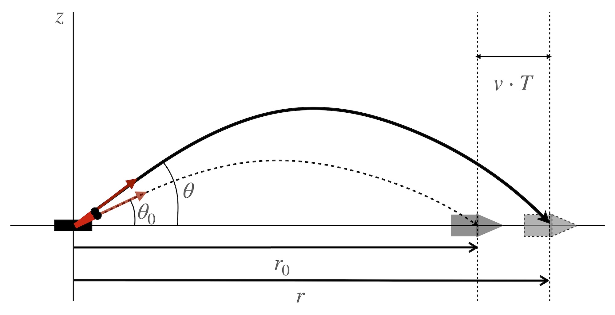
8.38.4.1 Free-Fall Projectile

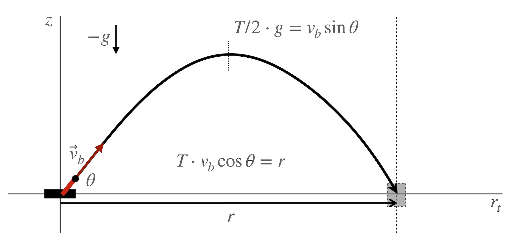
For this case, gravity is the lone force acting upon the projectile and is in the downward vertical direction. The projectile is launched at horizontal and vertical coordinates \((r_t,z) = (0,0)\) with speed \(v_b\) and initial vertical angle \(\theta\). The projectile returns to \(z = 0\) at a projected distance away in the horizontal plane, \(r_t = r\), called the range. The time to travel the entire range is \(T\).

Looking along the line of \(r_t\) from the gun to the target, the horizontal speed of the projectile is \(v_b\cos\theta\) and remains constant for the duration of the flight. The initial vertical speed is \(v_b\sin\theta\). However, this component of the velocity vector changes due to the downward acceleration of gravity. At the time \(T/2\) the shell reaches the apex of its trajectory as the vertical velocity reaches zero: \(\Delta v = 0 - v_b\sin\theta = -g\cdot \Delta t = -g\cdot T/2\). From this we find the total time of flight to be

\[ T = 2(v_b/g)\sin\theta . \]

The range \(r\) achieved from this value of \(\theta\) in time \(T\), assuming a return to the same initial altitude, will be

\[ r = v_b\cos\theta \cdot T = 2 (v_b^2/g)\cos\theta\sin\theta = (v_b^2/g)\sin 2\theta . \]

Hence, the maximum range of the gun is given by \(R \equiv v_b^2/g\), which occurs for \(\theta\) = 45 degrees, and the time of flight in terms of \(R\) is just

\[ T = 2(R/v_b)\sin\theta. \]

The maximum height the projectile achieves is

\[ h = \frac12 g(T/2)^2 = \frac12 \frac{v_b^2}{g}\sin^2\theta = \frac12 R \;\sin^2\theta . \]

With the above, we can write the equations for the particle’s trajectory in space:

\[ r_t(t) = v_b\cos\theta\cdot t , \\ ~\\ z(t) = v_b\sin\theta\cdot t - \frac12gt^2 \\ \]

or, in terms of the gun’s maximum range \(R\), and the total time \(T\) to reach the target,

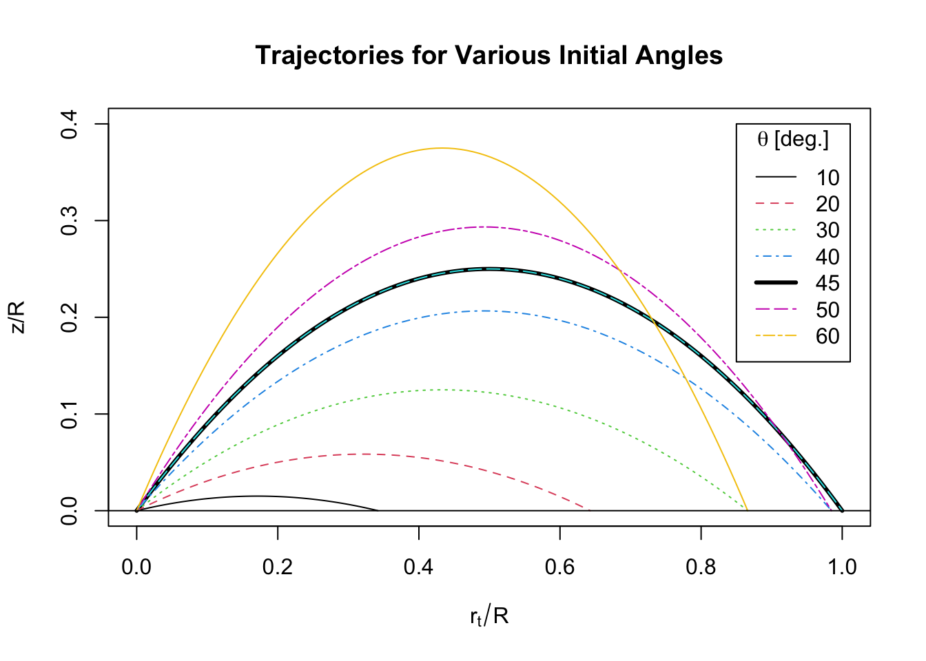
\[ \frac{r_t(t)}{R} = 2 \cos\theta\sin\theta \cdot \left(\frac{t}{T}\right) , \\ ~\\ \frac{z(t)}{R} = 2\sin^2\theta \cdot \left[ (t/T)-(t/T)^2 \right] . \]

For illustration, below is a plot of trajectories with firing angles between 10 and 60 degrees.

8.38.4.2 Effects of Air Resistance

The underlying assumption in the discussion so far is that gravity is the only force acting on the projectile. However, this would mean that it is traveling in a vacuum. But in reality a projectile fired at high speed near the earth’s surface will have another force acting on it in opposition to its motion through the air – air resistance, or drag.¹⁴⁰ For the high velocities we are discussing, this force is proportional to the square of the speed of the projectile. The constant of proportionality depends upon physical properties of the object and of the fluid through which it travels. In particular, the acceleration due to the drag force is characterized, to lowest order, by the equation

\[ a_d = \frac{F_d}{m} = k v^2 = \frac{\rho C_{d} A}{2m} \; v^2 \]

and is in the direction opposite to the velocity \(\vec{v} = v_{r_t} \hat{r_t} + v_z \hat{z}\). Here, \(\rho\) is the density of air, \(C_d\) is the so-called “drag coefficient”, \(A\) is the cross sectional area of the object transverse to the direction of motion, and \(m\) is the object’s mass. As one can imagine, this force/acceleration could be significant at high speed \(v\).

To see the effect, a small code can be written to illustrate. First, we introduce some constants:

g  = 32.17    # acceleration of gravity     [ft/s^2]
dt = 0.01     # "infinitesimal" time interval [s] 
vb = 1000     # initial speed of projectile [ft/s]

rhoAir = 0.0765        #  air density at sea level   [ lb/ft^3 ]
Cdrag  = 0.4           #  drag coefficient  (typical)
Ashell = pi*(16/2)^2   #  shell area      [in^2]
Wshell = 2500          #  shell weight    [ lb ]
fudge  = 1
k0     = rhoAir * Cdrag * Ashell/12^2 / 2 / Wshell * fudge  # [1/ft]

Rmax = vb^2/g      # in vacuum
zHat = vb^2/g/2    # in vacuum

Next, we give some initial conditions,

rt = 0
z  = 0
t  = 0

theta = 35*pi/180         # initial vertical angle of projectile
vrt   = vb*cos(theta)     # initial horizontal projectile speed
vz    = vb*sin(theta)     # initial  vertical  projectile speed
R     = Rmax*sin(2*theta) # range, in vacuum

and then we loop over consecutive time intervals computing acceleration and velocity at each step, and keep track of the longitudinal position \(r_t\), elevation \(z\), and time \(t\):

i=0
while(z[i+1] >= 0){
   i=i+1
# acceleration components :
   art = -k0 * sqrt( vrt^2 + vz^2 ) * vrt
   az  = -k0 * sqrt( vrt^2 + vz^2 ) * vz - g
# velocity components:
   vrt = vrt + art * dt
   vz  = vz  + az  * dt
# position components:
   rt[i+1] = rt[i] + vrt * dt
   z[i+1]  = z[i]  + vz  * dt
# time:
   t[i+1] = t[i] +      dt
}

Plotting our results, we find:

In the above image, the dotted red curve is the “in vacuum” solution of shooting the gun at a 45 degree angle. The solid red curve is the same, but for an initial angle of 35 degrees. The wide black curve is for our 35 degree initial angle, but with air resistance included. We can see that the effects of air resistance are significant.

As another illustration, a plot of trajectories is provided below for \(\theta\) = 45 degrees, over a range of values for the constant \(k\) that creates drag in our equations of motion.

So how would one go about using a slide rule to compute answers to such a scenario? First, we will assume that the slide rule is effective for a particular gun using a particular shell, etc. What we need to know is what horizontal range \(r\) and time of flight \(T\) is produced by each angle of elevation \(\theta\) of the gun. After all, it is the angle of elevation that will be dialed into the system before firing. In reality, this is something that would be measured on a firing range, and results tabulated for future use, thus incorporating all parameters of the real world. But to get a sense of how things go, we can use our equations above and prior variable values to perform a “loop” over a range of angles, producing curves of \(r\) and \(T\) as functions of \(\theta\). This is done here,

thetaCurve = seq(1,90,1)
j=0
rmx = 0
Tmx = 0
va  = 0
while(j<length(thetaCurve)){  # loop over angles
   j=j+1
   rt = 0
   z  = 0
   t  = 0
   vrt = vb*cos(thetaCurve[j]*pi/180)
   vz  = vb*sin(thetaCurve[j]*pi/180)
   i=0
   while(z[i+1] >= 0){        # track trajectory
      i=i+1
      art = -k0 * sqrt( vrt^2 + vz^2 ) * vrt
      az  = -k0 * sqrt( vrt^2 + vz^2 ) * vz - g
      vrt = vrt + art * dt
      vz  = vz  + az  * dt
      rt[i+1] = rt[i] + vrt * dt
      z[i+1]  = z[i]  + vz  * dt
      t[i+1]  = t[i]  +      dt
   }
   rmx[j]  = rt[length(rt)]      # final range
   Tmx[j]  = t[length(rt)]       # time of flight
}

va = rmx/Tmx  # ave. horiz. speed

Here are the resulting curves:

The last curve plots \(v_a(\theta) \equiv r(\theta)/T(\theta).\) The red vertical dashed lines are at \(\theta\) = 800 mils = 45 degrees, the angle for maximum range in vacuum, and the typical maximum angle possible for such guns. We see that with air drag, the maximum range occurs at an angle only slightly less than 800 mils for the initial ballistic speed of 1000 ft/s and our other chosen parameters. For higher initial speeds, the maximum range might be found at even smaller initial firing angles.

8.38.5 A Moving Target

An Example: Arbitrary Moving Target.

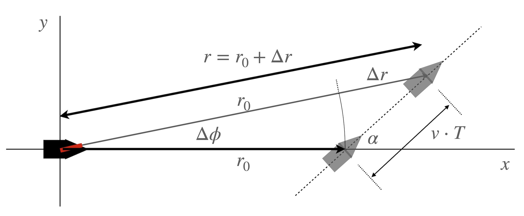
From Paul Ross’ notes on this slide rule, there is speculation that the rule was used in calculations involving “moving targets”. So let’s look at this for a bit. Consider an instantaneous coordinate system where the origin is maintained at the ship location, with the cannon being trained upon the target. From the ship’s frame of reference, the target is moving at speed \(v\) along a straight line path. At time \(t=0\), the target crosses \((x,y) = (r_0,0)\) with angle \(\alpha\) relative to the \(x\)-axis. We presume the distance \(r_0\) is known from rangefinder or radar measurements, and from a set of such measurements the speed \(v\) has been estimated. The gun is rotated in the horizontal plane by an angle \(\Delta\phi\) and the shell is fired at vertical angle \(\theta\), eventually reaching a point defined by polar coordinates \((r,\Delta\phi)\). The angles \(\Delta\phi\) and \(\theta\) need to be chosen so that the time \(T\) it takes the shell to reach \((r,\Delta\phi)\) is the same as the time it takes the target to reach the same point. For scale, large ships might move at speeds \(v\) of 10-40 mph = 15-60 ft/s, while their guns can easily fire projectiles at speeds \(v_b\) of 700-1600 mph = 1000-2500 ft/s.

From the above figure we can see that,

\[ r^2 = (r_0+vT\cos\alpha)^2 + (vT\sin\alpha)^2 = r_0^2 + 2r_0vT\cos\alpha + (vT)^2 \\ (r/r_0)^2 = 1 + (vT/r_0)^2 + 2\cos\alpha\;(vT/r_0) \\ \]

or

\[ \left[\frac{r(\theta)}{r_0}\right]^2 = 1 + \left[\frac{v\;T(\theta)}{r_0}\right]^2 + 2\cos\alpha\;\left[\frac{v\;T(\theta}{r_0}\right] \]

If we know values for \(v\), \(\alpha\), and \(r_0\) from previous measurements, and if we know the functions \(r(\theta)\) and \(T(\theta)\) of the gun, then in principle we can find a value of \(\theta\) that will satisfy the above equation. But, for this particular value of \(\theta\), the gun also needs to be aimed at the appropriate azimuthal angle, \(\Delta\phi\), at the time of firing. This angle is easier to ascertain through the use of our last figure:

\[ \sin\Delta\phi = \frac{\Delta y}{r} = \frac{v\;T(\theta)\cdot\sin\alpha }{r(\theta)} = \frac{v}{v_a(\theta)}\cdot\sin\alpha \]

or

\[ \cos\Delta\phi = \frac{r_0+vT(\theta)\cos\alpha}{r(\theta)}. \]

Note that the ballistic projectile speed will be much greater than the speed of the target in almost all circumstances (perhaps by a factor of 100 or so). Therefore we would expect \(\sin\Delta\phi\) to be relatively small.

Putting these two constraints together we can show that

\[ \frac{r(\theta)}{r_0} ~~~~~~ = \frac{[v/v_a(\theta)]\cos\alpha + \sqrt{1-[v/v_a(\theta)]^2\sin^2\alpha}}{1-[v/v_a(\theta)]^2} \\ ~\\ = \frac{[vT(\theta)/r(\theta)]\cos\alpha + \sqrt{1-[vT(\theta)/r(\theta)]^2\sin^2\alpha}}{1-[vT(\theta)/r(\theta)]^2} \\ ~\\ ~~~~~~~~~~~~~= \frac{\sin\Delta\phi/\tan\alpha + \cos\Delta\phi}{1-(\sin\Delta\phi/\sin\alpha)^2} ~~~~~~~({\rm for}~\alpha\ne 0). \]

Let’s next look at a couple of special cases.

8.38.5.1 Example 1: Receding Target Trajectory: \(\alpha\) = 0 degrees

An Example: Receding Target.

For the case where \(\alpha\) = 0, \(\Delta\phi\) will be zero – the target is moving directly away from the ship. We can see that starting from \((r/r_0)^2 = 1 + (vT/r_0)^2 + 2\cos\alpha\;(vT/r_0)\),

\[ (r/r_0)^2 = 1 + (vT/r_0)^2 + 2(vT/r_0) = (1+vT/r_0)^2 \\ ~\\ \frac{r}{r_0} = 1 + \frac{vT}{r_0} \\ ~\\ \frac{v \;T(\theta)}{r_0} = \frac{r(\theta)}{r_0} - 1 ~~~~~~ = ~~~~~~ \frac{\Delta r}{r_0}. \]

These last two combinations are ones that could be determined from settings on a slide rule with appropriate scales.

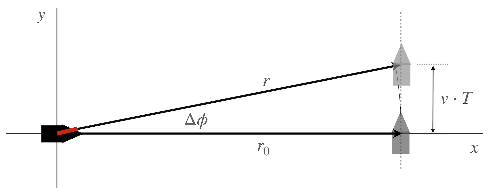
8.38.5.2 Example 2: Perpendicular Target Trajectory: \(\alpha\) = 90 degrees

An Example: Perpendicular Target Trajectory.

For this case, we have

\[ \frac{r}{r_0} = \frac{\sqrt{1-[v/v_a(\theta)]^2}}{1-[v/v_a(\theta)]^2} = \frac{1}{\sqrt{1-[v/v_a(\theta)]^2}} = \frac{1}{\sqrt{1-[vT/r]^2}}. \]

From here we may square and cross-multiply, and surmise that

\[ r^2-v^2T^2 =r_0^2 \\ ~\\ \frac{v^2\;T(\theta)^2}{r_0^2} = \frac{r(\theta)^2}{r_0^2} -1 ~~~~~~\approx~~~~~~ 2\frac{\Delta r}{r_0} \]

since we expect to have \(\Delta r \ll r_0\). We also see from geometry that

\[ \cos\Delta\phi = r_0 / r(\theta), \\ ~\\ \sin\Delta\phi = v \; T(\theta)/r(\theta) , \\ ~\\ \tan\Delta\phi = \frac{v}{r_0} \;\cdot\; T(\theta). \]

Note that for small values of \(\Delta\phi\),

\[ \Delta\phi \approx \frac{v\cdot T(\theta)}{r(\theta)} \approx \frac{v}{r_0}\cdot T(\theta). \]

And, correspondingly,

\[ 1-\cos\Delta\phi \approx 1 - (1-\frac12\Delta\phi^2) = \frac12 \Delta\phi^2 = \frac12 \left[ \frac{v\cdot T(\theta)}{r_0} \right]^2 , ~\\ 2(1-\cos\Delta\phi) \approx \left[ \frac{v\cdot T(\theta)}{r_0} \right]^2 . \]

So, in principle, one could align \(v\), \(T(\theta)\), \(r_0\), and \(\Delta\phi\) on a slide rule with appropriate scales and read off the values necessary to hit the moving target.

---

8.38.6 Special Scales Revisited

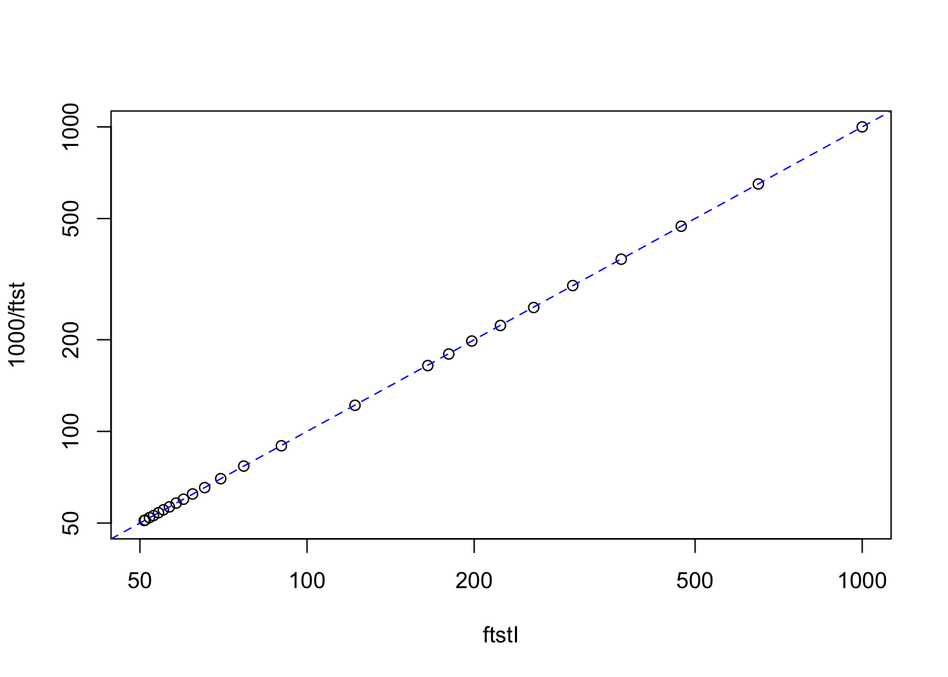
Having gone through all of the above, I went back to look at our “special scales” (1) and (12). Taking another look, I carefully re-tabulated values of Scale (1) directly off of Scale (8), a 20-cm log scale. More explicitly, I read a value of 1000 on (8) for a value of 60 mils on (1), 650 for 70 mils, …, down to 50.9 for 1540 mils. I repeated this process using Scale (17), an inverted 20-cm-decade scale on the back of the slide, where I took a value of 1 at 60 mils, 1.54 at 70 mils, …, up to 19.5 at 1540 mils. After inverting the second set and multiplying by 1000, a plot of the two against each other shows that the two processes line up, as they should when things have been read properly:

Angle   = c(seq(60,100,10),seq(110,150,10),seq(200,1500,100),1540)
ftstI   = c(1000,650,472,368,301,256,223,198,180,165,122,89.9,76.9,
            69.9,65.4,62.2,59.9,58.1,56.5,55.1, 54,52.9,52,51.1,50.9)
ftst    = c(1,1.54,2.12,2.72,3.32,3.92,4.49,5.05,5.57,6.08,8.21,11.15,13,
            14.3,15.3,16.05,16.7,17.2,17.7,18.1,18.5,18.9,19.2,19.55,19.62)
PLOTrng = c(50,1000)
plot(ftstI, 1000/ftst, xlim=PLOTrng,ylim=PLOTrng,log="xy")
abline(a=0, b=1, lty=2, col="blue")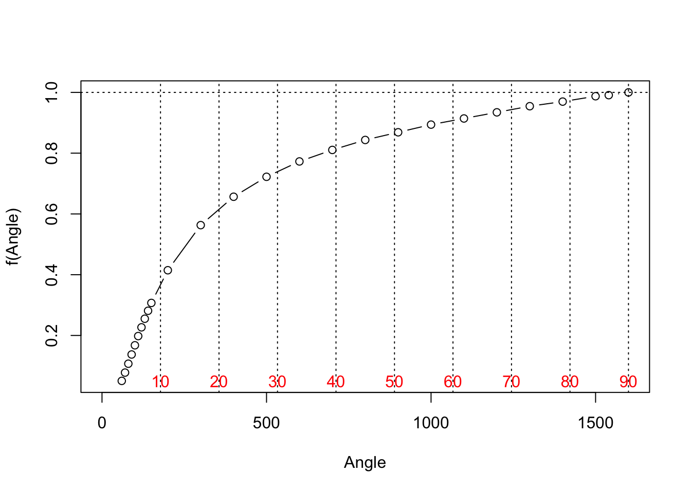

So let’s give our function \(f\) a value of “1” at an angle of 90 degrees. Then,

ffin    = c(ftst,19.8)/19.8
AngMils = c(Angle,1600)

Hence, we can show a plot of the function \(f\) where \(f\) is on Scale (12) (in degrees) and \(1/f\) is on Scale (1) (in mils).

plot(AngMils,ffin,typ="b", xlim=c(0,1600), xlab="Angle", ylab="f(Angle)")
abline(h=1,v=Ang[-2]/90*1600,lty=3)
text(Ang[-2]/90*1600,0.05,Ang[-2],col="red")

Next, we note that if we plot \(f^2(\theta)\), which would correspond to values on the 10-cm-decade scales, then the values “very roughly” conform toward our curve \(T(\theta)\) when scaled to the value of \(T(90^\circ)\), as shown next:

The value of \(T(90^\circ)\) using our ballistics parameters is 58.55 seconds and, remember, the gun likely would never (and probably can’t) fire at an angle greater than 45 degrees (red vertical dashed line). Note, too, that one curve of “1-cos” had a factor of about 60 out front, differing from \(T(90^\circ)\) by about 2 %. Our present analysis of the slide rule scales does not provide any exact match to our expected ballistic behavior using lowest-order physics, but it is still fairly suggestive. It is likely that the values on the slide rule would take into account a range of other effects that are important, especially for low and high firing angles, which could have been found empirically.

So we appear to have a special function \(R(\theta) \equiv f^2 = T(\theta)/T(90)\) that provides us with the time of flight for various initial angles. What we need next is the function \(r(\theta)\) on the rule as well. We know that in vacuum the range – call this \(D\) here – would be \(D(\theta) = (v_b^2/g)\sin\theta\cos\theta.\) So, in the plot that follows, we present (a) the function \(r(\theta)\) from our earlier analysis, using \(v_b\) = 1000 ft/s, etc.; (b) the range in vacuum \(D(\theta)\); (c) the relative difference \((D-r)/r\) between the two (in percent); and, (d) the function \(D\) with a straight scaling by a factor of 0.85 in order to make \(D\) line up better with \(r\).

This tells us the function \(r(\theta)\) will still closely resemble a “sine times cosine” scale, which we earlier deemed Scale (6) to be. So perhaps Scale (6) truly is our function \(r(\theta)\). In the initial analysis of Scale (6) I was able to line up a \(\sin\theta\cos\theta\) scale very precisely, but an over all “scale factor” would simply result in a displacement of the scale on the rule. As noted much earlier, the trig scales on the slide are not aligned with any particular logarithmic scale on the slide rule in the traditional manner.

However, it is interesting to point out that on the slide, Scale (6) – the “sine times cosine” scale – has its value of 45 degrees lining up with just under “26” on Scale (3) – a 10-cm-decade log scale. This suggests to me that, perhaps, the maximum range of the gun system is about 26 – maybe in units of 1000 feet? – and that perhaps distances in kft are read off of Scale (3), tied to the angles shown on Scale (6). This would be consistent with our use of \(v_b\) = 1000 ft/s in our earlier calculations, if the drag parameter \(k\) is adjusted to be about 8.5 \(\times 10^{-6}\)/ft. This actually is the reason the parameter was chosen to have this value in our earlier calculations, while still keeping it consistent with typical gun and shell parameters.

So, for now, let’s suppose Scales (12) and (1) represent \(R(\theta) = T(\theta)/T(90)\) and \(1/R(\theta) = T(90)/T(\theta)\), respectively. Note that if the time is measured in units of minutes, then \(T(90)\) is very close to 1. And also suppose that Scale (6) is to be used directly for \(r(\theta)\). How would these scales get used? Well, for \(\alpha\) = 90 degrees,

\[ \tan\Delta\phi = \frac{v\;R(\theta)\;T(90)}{r_0}, \\ ~\\ \frac{v}{r_0} \cdot T(90) = \frac{\tan\Delta\phi}{R(\theta)}. \]

This last ratio is one that could be set up on a slide rule to determine what \(\Delta\phi\) to use for a chosen value of \(\theta\), since the parameters \(v\) and \(r_0\) are measured, and \(T(90)\) is given by the gun system.

Can We Now Work a Problem?

Let’s consider an example using the following parameters. A target traveling at \(v\) = 22.7 miles per hour = 2000 ft/min perpendicular to the gun’s line of sight is determined from rangefinder measurements to be \(r_0\) = 7250 ft = 1.37 miles away.

The distance in question is within the maximum range of the gun (26 kft for \(\theta\) = 45 degrees). To reach \(r_0\) the gun would require an initial angle of \(\theta \approx 8^\circ\). Thus, an intermediate vertical firing angle of, say, 10 degrees is selected. From our plot of \(R(\theta)\), we find that \(R(10)\) = 0.137. If we use \(T(90)\) = 1 minute, then the necessary azimuthal angle required to strike the target is given by

\[ \Delta\phi = \tan^{-1}\left[ \frac{v\cdot T(90)}{r_0}\cdot R(\theta)\right] \]

which gives \(\Delta\phi\) = 38.6 mils, using a computer.

We now use the Byoutou slide rule to perform the calculation. With the slide reset such that scales (2) and (3) – both 10 cm logarithmic scales – are aligned, we find that scales (12) and (7) are also aligned at the right-hand end at common values of “1”. So by aligning two numbers on (2) and (3) to form a ratio, then this will automatically produce a ratio between the \(R\) function on scale (12) and the tangent function on scale (7), just what is needed.

The biggest concern, as usual, is the placement of the decimal point. This is particularly important using this slide rule as there are scales that extend beyond two decades in length. Estimating \(vT/r_0\) from our numbers we find that it is approximately 0.3. So, to proceed, we set 72.5 (\(r_0\)) on scale (3) against 2 (\(v\)) on scale (2). This ensures that the right index of the slide does not move left by more than one decade (keeping the intermediate result near 0.3). Then, finding \(\theta\) = 10 degrees on scale (12) using the cursor, we find under the cursor on scale (7) the value \(\Delta\phi\) = 38 mils.

A Byoutou calculation on the Hemmi slide rule.

8.38.7 Concluding Remarks

Our Final (for now) Analysis:

Scale	Range (L-to-R)	“Type”
V	100 - 400	A
“L”	0 - 10	L/cm
(1)	1600 - 60	RI
(2)	0.3 - 10	A
(3)	3 - 100	B
(4)	3 - 90	S
(5)	3 - 87	T
(6)	3 - 45	CS
(7)	3 - 800	T
(8)	50 - 1000	D
(9)	60 - 30	2(1-C)I
(10)	30 - 20	(1-C)I
(11)	110 - 1600	S
(12)	10 - 90	R
(13)	2 - 50	B
(14)	87 - 3	TI
(15)	90 - 3	SI
(16)	3 - 1000	B
(17)	21 - 1	CI
(18)	5 - 100	C

Well this has been a fascinating journey and I have learned a lot. While I believe we have interpreted fairly successfully all of the scales on the slide rule, and we have used a few of them to perform a relevant ballistics calculation, what I didn’t learn, however, are all of the ways to use the Byoutou slide rule. Certainly we can easily write down standard equations and use the standard functionality of the rule to perform many calculations. But what particular procedures were intended by the slide rule designers? And are our interpretations of the “special scales” that we have investigated even close to what the designers had in mind? What is the intended purpose of the “V” scale? There are many other questions remaining. Including, what are the units being used? My use above of English units of feet and seconds gives results that are in the realm of reality, and it should be noted that the traditional Japanese shaku unit of length is 11.93 inches long. Using units of meters and seconds (with \(g\) = 9.8 m/s\(^2\) as opposed to 32 f/s\(^2\), and so forth) should work the same, as the relationships would be the same and the scales would be used the same way. But the range of values on the scales of the rule are consistent with feet and seconds/minutes, and with the gun parameters of the mid-1940s.

Scales (1) and (12) appear to align with basic time-of-flight calculations, but some details of their functional form remain unaccounted for. Is this just a result of our simple model not accounting for the real world, or is it a complete misunderstanding of the scales?

There could be other factors that could be put into a more complete ballistic model, especially at small angles, or even at large range. For instance, we could include

• additional rotational motion of the cannon before firing, causing an azimuthal component of the shot, thus producing an additional small angle in its trajectory.
  
• the rifling of the shot through the cannon barrel in conjunction with air resistance, generating rotation of the shell and thus producing an additional drift angle.
  
• the curvature of the earth for long-range travel.
  
• etc.

Such considerations could have and most surely would have been built into the design of the system, and compensated for in the scale used in (1) and (12), and perhaps (9) and (10). Then again, perhaps we are misinterpreting what functions are represented by these scales. But our example problem above leads me to believe that we are at least on the right track.

And when would one use the three scales on the back of the slide? Are they just there for general computational work? Sounds likely to me. And for which problems would one take out the slide and reverse it to use scales (14) and (15)? I think this could become obvious with just a little more effort put into this subject. There are many mysteries to me about this rule; many standard scales, but very much an “expert’s” slide rule. I will no doubt continue to think about the scales on this slide rule and continue to comb for new information related to it. If new evidence is found or new information uncovered, this article will be updated accordingly.

The folklore surrounding this slide rule seems to suggest it may have been used in the training of naval officers. It seems to me that when trying to teach such a subject one may wish to differentiate the azimuthal angles (using mils, say) from the elevation angles (by using degrees, say). Such differentiation would not be necessary for an experienced officer, but perhaps would have been useful for a more general introduction to the problems being taught. The Byoutou with its textbook referring to the various labeled scales would allow the less experienced to learn about many different applications without needing to be proficient in general slide rule use. Clearly, with a total of almost 20 individual scales on the slide rule, and an implied “slide inversion” required for certain calculations, there must have been a slew of problems with which it was meant to help solve. Which begs the question,

“How do you Byoutou?”

---

A nice overview of naval and military ballistic topics can be found here:

• Fire Control Fundamentals, NAVPERS 91900, U.S. Navy, 1953.

• Wikipedia article on The Japanese 46 cm/45 Type 94 naval gun.

• Elizabeth R. Dickinson, “The Production Of Firing Tables For Cannon Artillery”, Report No. 1371, Ballistic Research Laboratories, Aberdeen Proving Ground, Maryland, November 1967.

I would like to give special thanks to George Anderson for his continuous support in this endeavor, particularly his contributed documentation regarding military ballistics and the development of firing tables.

---