2.6 Summary
We have found that the base of the natural logarithm, \(e\) = 2.7182818…, can be computed to very high accuracy in a straightforward way, as can the values of the natural logarithm \(\ln x\) of an arbitrary number \(x\), by using a Taylor series (or, “power series”) approach. Such calculations could take a very long time in the days before high performance electronic computers, yet, as we’ve seen, books of tables of such results were constructed centuries ago by hand, pen, and paper using such techniques. Today, values of logarithms can be obtained directly on your smart phone.
In addition, we found that our natural base raised to any power, \(e^x\), can also be computed as well using the general power series derived earlier:
\[ e^x = 1 + x + \frac{1}{2}x^2 +\frac{1}{6}x^3+\frac{1}{24}x^4 +\frac{1}{120}x^5+ ... \]
In fact, using another of our earlier results, we see that any number \(b\) raised to a power \(x\) can be written in terms of the exponential function as
\[ b^x = e^{(x\cdot\ln b)} \]
and so any number raised to any power can be computed using the functions developed here. The exponentiation of any base number, \(b^x\), can be considered a version of the general exponential function \(e^x\) with a properly scaled argument, where \(e^x\) is the function whose value grows at an instantaneous rate that is equal to the function’s instantaneous value.
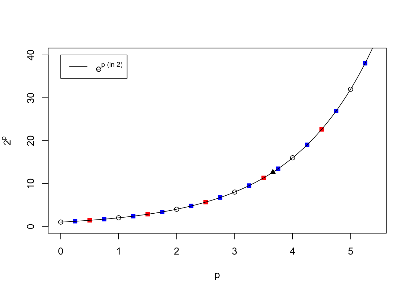
Take the graph we constructed in the previous chapter where we plotted \(2^p\) for various values of \(p\), which included \(p\) = 0, 0.25, 0.5, … 4.75, 5. To emphasize our point, we re-plot these results below, along with a curve of \(e^x\) which is a calculation based upon our Taylor series formulas, but identifying \(x = p\times\ln 2\):
And finally, since we know how logarithms from different bases are related to each other, we can compute logarithms \(\log x\) which use Base 10 from the logarithms \(\ln x\) computed using Base \(e\) through the formulas we developed:
\[ \ln (1+x) = x - \frac{1}{2}x^2 + \frac{1}{3}x^3 - \frac{1}{4}x^4 +\frac{1}{5}x^5 - ... ~~~~~~~~~~~~~~ {\rm for} ~-1<x\le 1, \\ ~\\ ~\\ \\ \log x = \frac{\ln (a/10)}{\ln 10} + n+1 ~~~~~~~~~~~~~~ {\rm where} ~~ x=a\times 10^n, ~~1<a\le 10, ~~ n=integer. \]
The point of this entire discussion has been to describe a process through which the common logarithm of an arbitrary number can be computed to the accuracy required for implementation on a slide rule. We developed formulas that can be used to compute logarithms \(\log x\) that use Base 10, derived from logarithms \(\ln x\) using Base \(e\). We have not described the actual historical path of the development of logarithm calculations, and the computational algorithms shared above are not necessarily (almost guaranteed not to be) the most computationally efficient means for attaining values of logarithms. But hopefully the reader has gained an understanding for what is involved in such calculations as well as an appreciation for the work that it must have taken to arrive at values of logarithms in the days before the modern electronic computer.
Now that we’ve gone over the essentials of logarithms and methods for computing their values, let’s see how this is all put to use on the slide rule.