2.2 The Natural Logarithm

We want to find a mathematical function \(f(x)\) for values of \(x>0\) that can be evaluated in a straightforward way, and that has the properties of a logarithm that were discussed in the previous chapter. For instance, the function would need to have the following properties:

• The logarithm of 1 must be zero for any choice of base. Hence, \(f(1) = 0.\)
  
• The function should be positive for values of \(x\) greater than one, and negative for values of \(x\) less than one: \(f(0<x<1) < 0; ~~ f(x > 1) >0.\)
  
• As \(x\) approaches zero from the positive side, the function should approach negatively infinite numbers: \(f(x)\rightarrow -\infty\) as \(x\rightarrow 0.\)
  
• And, as \(x\) gets more and more positive, the function should tend toward positive infinity: \(f(x)\rightarrow +\infty\) as \(x\rightarrow +\infty .\)
  
• Lastly, but perhaps most importantly, since the logarithm of a product of two numbers must be the sum of the logarithms of the two numbers, we must have: \(f(a\times b) = f(a) + f(b).\)

It turns out that the area under a specific geometrical figure, which can be accurately computed through the use of calculus, has the above properties and hence can be used to define a natural logarithm. This may seem like a very strange approach toward defining a logarithm which is, after all, an exponent applied to a base number, a seemingly unrelated mathematical exercise. But we’ll see that for one particular curve, these two operations have a remarkable connection and the power of calculus allows us to compute the answers in a straightforward way.

The curve in question is that of a hyperbola. The standard equation in terms of two variables \(u\) and \(v\) for a general hyperbola is

\[ \left( \frac{u}{a}\right)^2 - \left( \frac{v}{b}\right)^2 = 1 \]

where \(a\) and \(b\) are constants. As an example, suppose \(a=b=\sqrt{2}\). We get \(u^2 - v^2 = 2\), which is shown in the following plot:

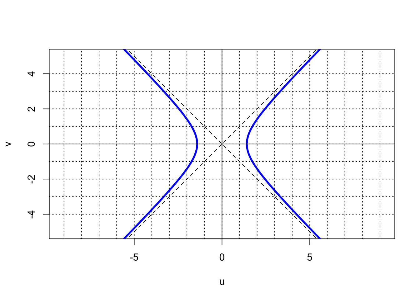
Notice how this relationship between \(u\) and \(v\) is not a function, as there are two values of \(v\) for each value of \(u\). There is also a region within which there are no combinations of real values of \(u\) and \(v\) that satisfy our equation. However, if we now rotate the figure by 45 degrees, we will arrive at a condition where \(v\) is a function of \(u\). Rotating by 45 degrees is equivalent to transforming the coordinates according to

\[ u \longrightarrow (~~u + v)/\sqrt{2} \\ v \longrightarrow ( -u + v)/\sqrt{2} \]

which transforms the equation \(u^2-v^2=2\) into

\[ u^2 - v^2 = 2 ~~~~\longrightarrow~~~~ (u^2 +2uv+v^2)/2 - (u^2 - 2uv +v^2)/2 = 2,\\ 4uv = 4, \\ ~~{\rm or}\\ u\cdot v = 1. \]

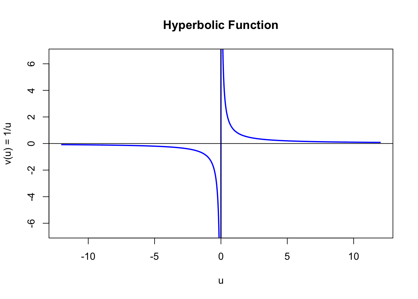
The equation of our new hyperbola becomes \(u\cdot v = 1.\) We see that this can be interpreted as a function \(v\) of the variable \(u\) where \(v(u) = 1/u\), as shown below. The function is undefined for \(u=0\), and tends to \(\pm\infty\) as \(u\) approaches zero from the right or left sides.

If we take the branch of our hyperbolic function for positive values of \(u\) we find, after a bit of inspection, that our properties of a logarithm can be met by defining a new function that is evaluated by finding the \(area\) between the hyperbolic curve and the horizontal axis. The area in question is shown below:

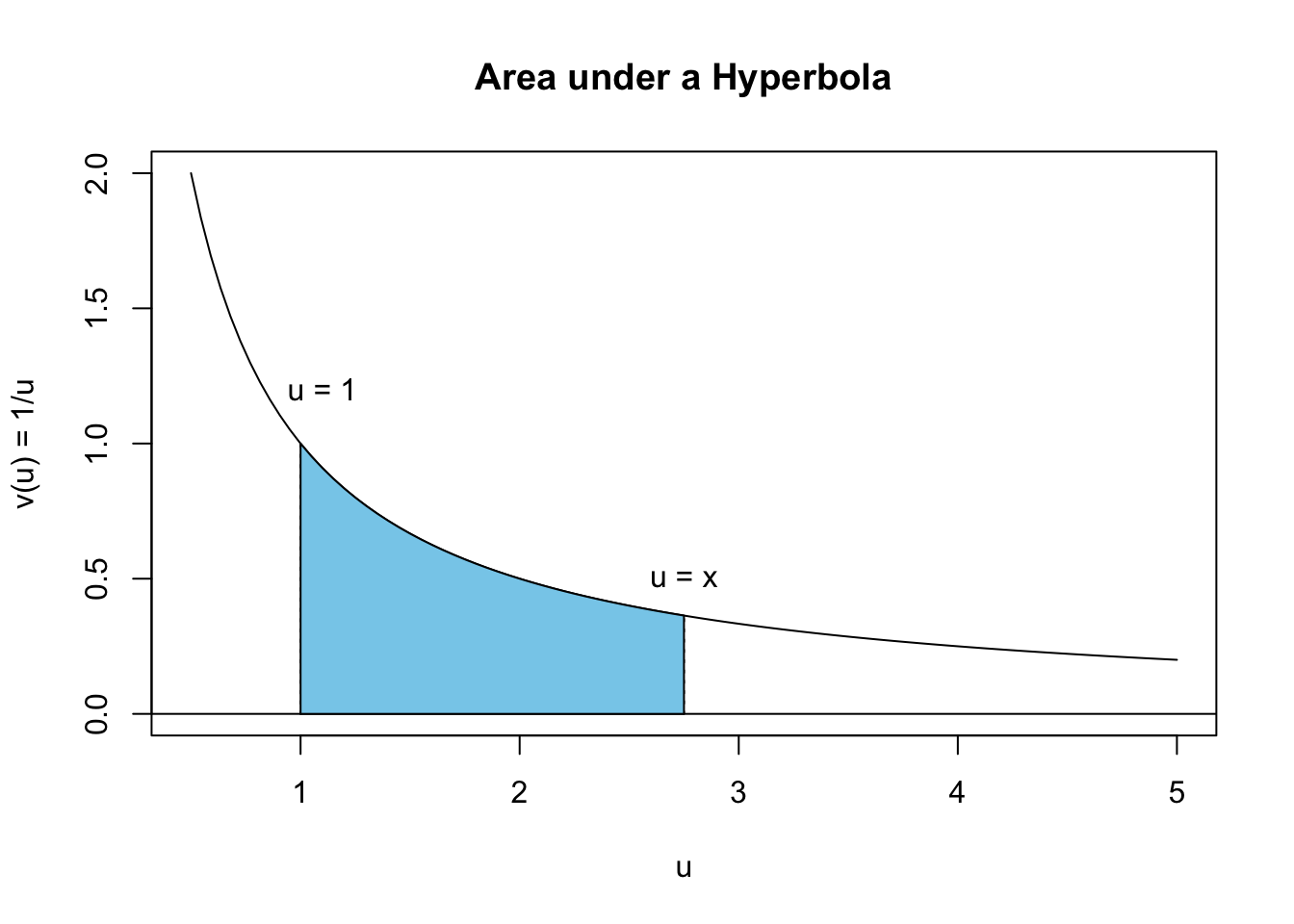
The shaded area always starts at \(u=1\) and stops at an arbitrary value \(x\), and so yields a function of \(x\), call it \(f(x)\). This function, therefore, can be computed using calculus by performing the following integration:

\[ {\cal Area} = f(x) = \int_1^x \frac{1}{u}\;du. \]

This integral has all the properties of a logarithm as we have listed previously. First of all, it obeys the rule of a logarithm in that the logarithm of \(a\times b\) is equal to the sum of the individual logarithms of \(a\) and of \(b\):

\[\begin{eqnarray*} f(a\times b) &=& \int_1^{ab} \frac{1}{u}\;du \\ &=& \int_1^{a} \frac{1}{u}\;du + \int_a^{ab} \frac{1}{u}\;du \\ &=& \int_1^{a} \frac{1}{u}\;du + \int_1^{b} \frac{1}{u}\;du ~~~~~~~({\rm replacing}~u \longrightarrow u/a)\\ &~& ~~ \\ &=& f(a) + f(b). \end{eqnarray*}\]

Secondly, for \(x\) = 1 the integration range will have zero length and hence \(f(1)\) will be zero. For values of \(x<1\) the integral will be negative, just as logarithms are negative for \(x<1\). That is, if \(x=a\) where \(0<a<1\), then \(\int_1^a = -\int_a^1\) and so the integral will have a negative value. In addition, the integral goes to \(-\infty\) as \(x\) approaches 0 and to \(+\infty\) as \(x\) approaches \(+\infty\). The function \(f(x)\) given by the above integral has all the basic properties of a logarithm.

For this reason, this integral represents a natural logarithm and is given the designation \(\ln x\) with the formal definition,

\[ \ln x \equiv \int_1^x \frac{1}{u}\;du. \]

It is quite remarkable that a well-defined mathematical function, formed from an analytical representation of a geometrical object, was found that exhibits all the properties of what had become known as a logarithm. But now, with a functional form identified, the techniques of calculus, developed in the late 1600s, can be employed to further analyze this function and its properties, permitting the direct computation of values of logarithms to high accuracy.