8.30 Gauging Electro Rules
Originally posted: 2023 Dec 14
Of the many Specialty Slide Rules that emerged during the first half of the 20th Century, one of the more common was a style used for general calculations in the electrical trades. As the world was becoming “electrified” during this period, the “Electro” slide rule became a standard tool of the engineers and linemen who were laying out the early electrical grid, wiring homes, buildings, and neighborhoods, and connecting rural communities.
The two basic types of calculations that were performed using these rules were (a) voltage drop through lengths of conductor and (b) power efficiency of generators (or “dynamos”) and motors. A standard slide rule could, of course, be used for such calculations, but the effort required was simplified when the slide rule had built-in conversion factors and scales labeled just for these purposes. These rules were not meant to compute quantities found in the more modern “electronics” engineering field, where high-frequency alternating currents are involved with more complicated issues such as inductance and impedance at play. Rather, the electro slide rules were used for direct current (DC) calculations, or low-frequency alternating current (AC) circuitry as might be found in the home.
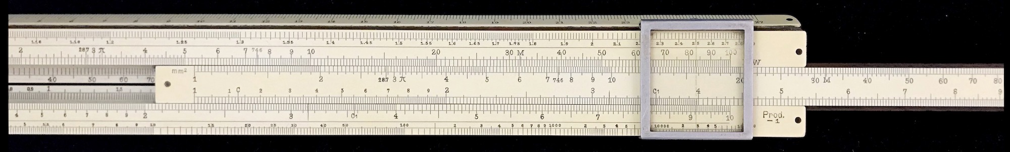
A nice example of an electro slide rule, the Faber-Castell 378, from 1913-14, is shown below.
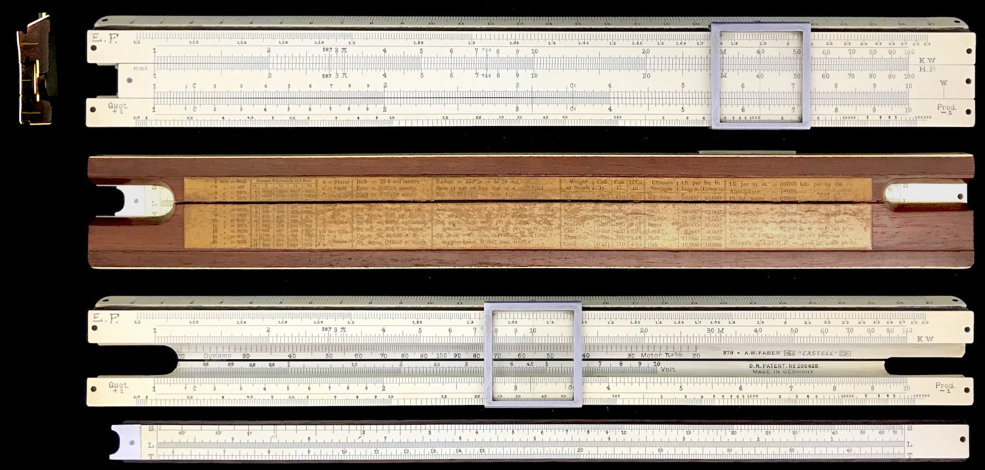
For the most part the scales are just the standard A, B, C, and D scales (with S L and T on the back of the slide), but with scales labeled “Dynamo/Motor” and “Volts” embedded in the well of the rule. It also has two Log-Log scales on the front, one on the top and one on the bottom. Faber-Castell introduced their first electro rule in about 1903-05, the Model 368. By about 1910, their new Model 378 was introduced, which was produced for nearly 3 decades. Model 368 was the first mass-produced slide rule by Faber-Castell to have log-log scales. (Keuffel and Esser in the US, for contrast, introduced their first log-log slide rule, the general-purpose Model 4092, in 1909.) The Models 368, 378, and 398 set the standard for many future electro rules from other makers, with only nuanced differences. The only electro rule manufactured by a major US maker was K&E’s Model 4133, which takes a slightly different approach that will be discussed below.
But to proceed, let’s talk a little about electric circuits and then see how an electro rule would have been used in the field.
8.30.1 Simple Electrical Circuit
If we consider an electrical circuit made up of a voltage source, some resistive elements (light bulbs, an electric stove, etc.), and wiring connecting them, then a simplified circuit might look like this:
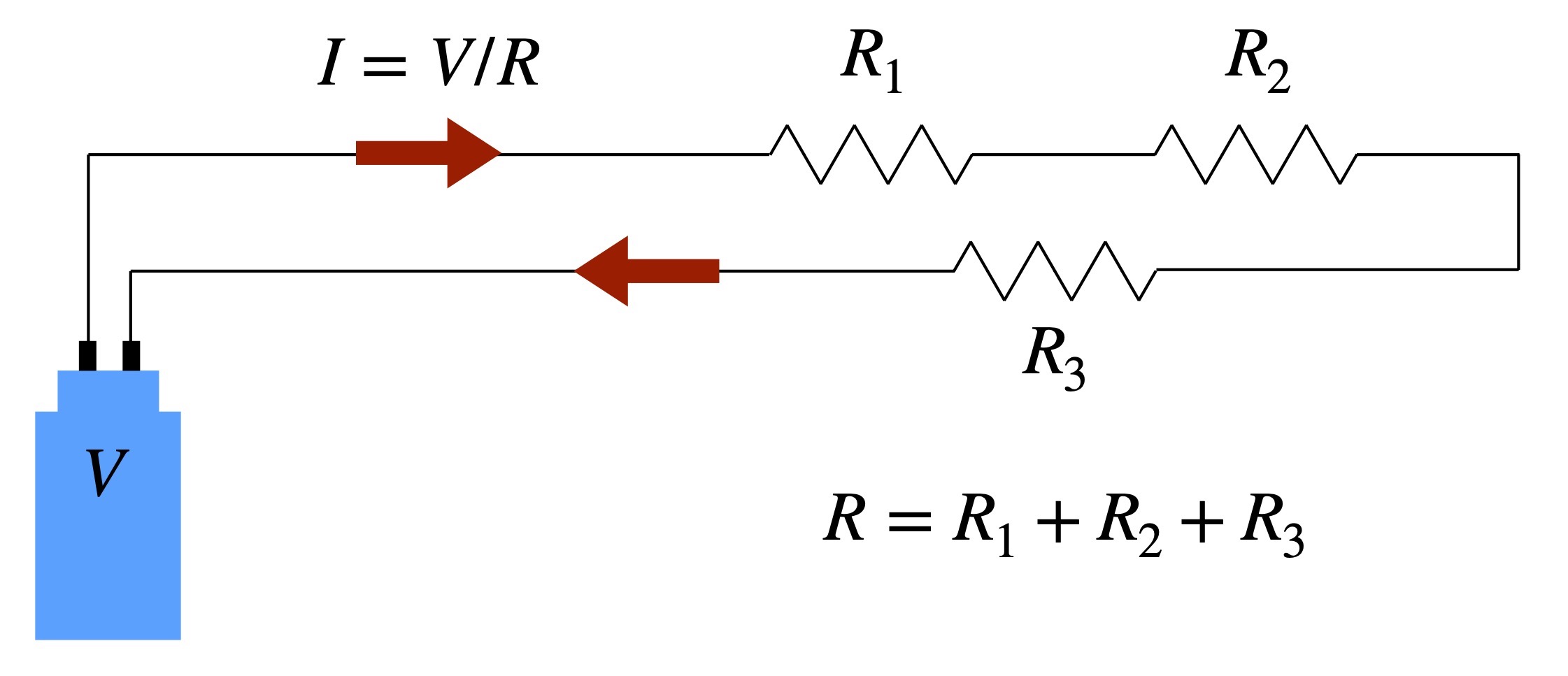
Consider a source of electrical current that is maintained at a set voltage, \(V\). This could be from a battery, or in the case of a low frequency AC system as in the home, it could be at an electrical outlet for instance. The electrical potential (voltage) at other points around the circuit will depend upon the “electrical resistance” of the items along the path. A light bulb might have a resistance of 120 Ohms, while an electric hair dryer might present a resistance of only 10-20 Ohms. An item with less resistance will allow current to flow more easily through it for the same set voltage. The entire resistance \(R\) of the items along this single circuit will be the sum of all the individual resistances along the path, and the total current drawn by the circuit will be \(I = V/R\), where \(I\) is in Amperes, \(V\) is in Volts, and \(R\) is in Ohms. This simple relationship, usually written as \(V = IR\), is called Ohm’s Law. In essence, the voltage at a point gives the potential for moving a charge through a “downstream” resistance. Once passed through this resistance, there is less potential for moving through further resistance encountered “downstream” along the path. At the completion of the path, at the battery or “voltage source”, the potential is returned to its original value.
8.30.2 Voltage Drop
In our circuit example above, the total resistance \(R\) is equal to the sum of the individual resistances \(R_1\), \(R_2\), etc. The current flowing through each item will be the same, namely \(I\), but the more total resistance the more slowly charges can pass through the circuit. The electrical potential across each resistive element will change by an amount \(\Delta V_i = - I\cdot R_i\) for the \(i\)th item in the circuit. This change is called the voltage drop across the element. The sum of all the voltage drops across all the elements plus the voltage \(V\) supplied at the source must all add up to zero. This relationship is called Kirchoff’s Law.
One consequence of Kirchoff’s Law and Ohm’s Law is that as we add elements to the circuit in a serial fashion, the total current will be reduced, so long as the source voltage is held constant. For example, if we have a light bulb in the circuit that burns at a particular brightness, then if we add a second similar light bulb into the circuit in series with the first, then each light bulb will burn at less than this brightness, as the circuit will draw less current due to the increased resistance. This is one reason that parallel circuits are used in homes and buildings.
The standard “introductory physics” approach has been taken up to this point in our discussion, where we neglect the resistance of the wires that connect our various resistive items. But, as we all know, the wires themselves are resistive as well, and hence they will contribute to the voltage drop along the circuit. On a high school physics lab table, the wires are short and their resistances are small enough to ignore, but in cases where wires run many feet, yards, or miles, the resistance can become significant. In such a case, just how resistance builds up along a wire or cable needs to be taken into account in the calculations of such systems.
8.30.2.1 Resistivity
Wires are made of conductive material which will have a certain amount of electrical resistance. And, the longer the wire the more resistance will be present. Additionally, the resistance of a wire will depend upon its cross-sectional area – in a thicker wire, the currents can “spread out” and hence less resistance is met for the conduction of current. Therefore, the actual resistance of a wire of length \(L\) (meters, say) and cross-sectional area \(A\) (square meters, say) is given by the relationship
\[ R = \rho \; \frac{L}{A}. \]
where the proportionality constant \(\rho\) is called the resistivity of the conductor. We see that the total resistance of a wire of a certain length can be adjusted by choosing a different cross section for the wire being used. Since the resistance is given in units of Ohms, and \(L/A\) has units of 1/m, then the unit of resistivity is Ohm-m (Ohm times meter). Other things affect resistivity of materials, such as copper, used in electrical applications – temperature is a common factor, and so corrections for temperature might be found on some of the electro slide rules.
8.30.2.2 A Voltage Drop Calculation
While resistivity has units of “Ohm - meters”, wires do not have dimensions measured in meters, of course. So the electro rules are to be used with a particular set of units assumed. For example, on our Faber 378 rule above, the A scale is associated with currents in units of 10 A and lengths in units of 10 m, typical orders of magnitude dealt with by electricians. On the B scale we associate wire cross-sectional area in units of 10 mm\(^2\). Diameters of a few millimeters are commonplace. Constants like \(\pi\) and \(\rho\) are then typically incorporated either into the Volt scale in the well of the rule, or as various Gauge Marks on the slide rule scales.
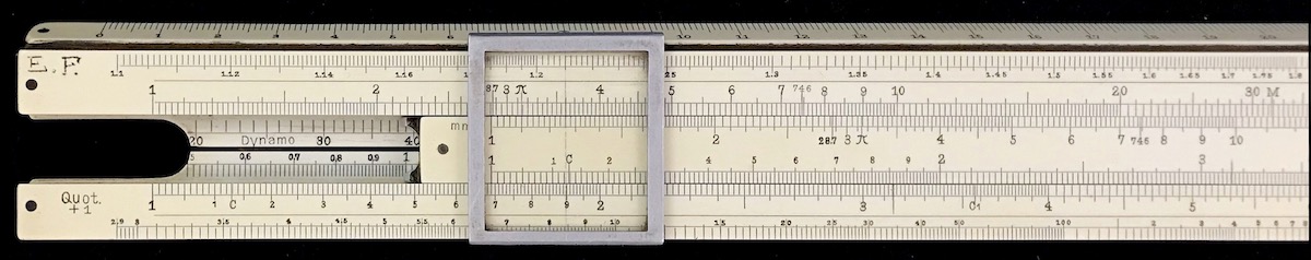
Let’s suppose we want to find the voltage drop through an electrical power line of length \(L\) = 15 m length using our Faber-Castell 378. The line contains two wires, one to the device we want to power, and one to return the current back to the source. (The “positive” and “negative” wires, say.) Each round wire is 4 mm in diameter and, for our example, is carrying 24 A of current. The voltage drop through the wires from the source to the load and back is
\[ \Delta V = 2\rho\cdot\frac{I\cdot L}{A} \]
where the factor of two takes care of the two wires, each of length \(L\), to and from the load. Our wire’s cross-sectional area is \(A=(\pi/4)\cdot 4^2\) = 12.6 mm\(^2.\) So, to perform the calculation on the slide rule, we line up the 1 on B with the 2.4 on A (24 in units of 10 A). Then, move the cursor to 1.5 (15 in units of 10 m) to do the upper multiplication. Finally, we divide by the area 12.6 by lining up 1.26 (12.6 in units of 10 mm\(^2)\) with the cursor. The result of the calculation is now found on the “Volt” scale in the well of the slide rule, using the metal edge of the slide as a cursor. This scale has the resistivity of copper built in, as well as our special factor of two for the two wires.134 As shown in the image below, we get a voltage drop of 1.0 V. By computer, we find:
dV = 1.014 V.
8.30.3 Wire Gauge
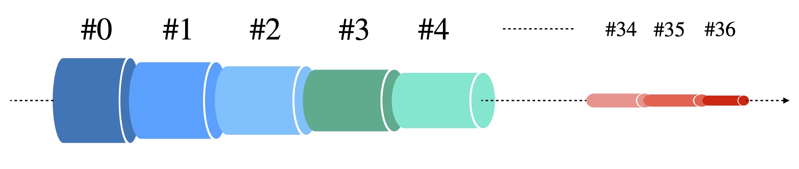
As noted, when laying out an electrical system the wires themselves will reduce the voltage at the final device to be powered. To meet the requirements of the device, the dimensions of the wires needed to be chosen to minimize the voltage drop to an acceptable level. Over the centuries, wires have been manufactured with a variety of “gauge” systems, which designate the thickness of a wire.135 While variations existed (and exist) around the world, a wire-sizing standard named the Brown and Sharpe wire gauge (based upon a sheet metal gauge system at the Brown and Sharpe Mfg. Co., Providence, RI, USA) was established in the US in 1856 to regulate the thickness of conductive wires made from nonferrous metals and we will use this as our example wire gauge system. The B&S standard, also called the American Wire Gauge (AWG) standard, has a total of 40 standard sizes, called #0000, #000, #00, #0, and #1 through #36, which get progressively smaller with larger gauge number. The progression of wire diameters, it turns out, is logarithmic in nature, as we will show below. In the production process, metal is annealed and extruded, or drawn through a set of dies, creating wires of successively smaller size. Each passage through a die gives the same relative reduction in diameter as the previous die. In the B&S standard, this reduction is about 11%, a limit found to reduce wire breakage during their process.
8.30.3.1 Brown and Sharpe Gauge
In the B&S/AWG system, there are 39 such extrusions which thus yields a total of 40 different wire diameters. A #0000 (pronounced “aught four”) wire has a diameter of 0.460 inch (460 mil) – 11.684 mm – while a #36 ( pronounced “number 36”) wire has a diameter of only 0.005 inch (5 mil) – 0.127 mm. The ratio of the range of wire size, 5/460 = 1/92, gives the overall reduction of wire diameter for the 40 different sizes in the system. This tells us that starting with #0000, to get to #36 requires a reduction at each of the 39 steps by a factor of \(1/\sqrt[39]{92}\) = 1/1.12293 = 0.89053.
Therefore, starting with Gauge #0000 wire at 460 mil = 11.684 mm diameter, for example, we see that the diameters of the other gauges are given by
\[ d = (11.684~{\rm mm})\times(0.89053)^{AWG+3},~~~~{\rm or,} \\ = (8.251~{\rm mm})\cdot (0.89053)^{AWG} \]
where \(AWG\) is the gauge number (Nos. 1, 2, and so forth; the “aught” gauges have zero or negative exponents). And from this formula, we can produce the diameters of wires in the AWG (B&S) system:
##         #0000  #000   #00    #0
## AWG      -3.00  -2.00  -1.00   0.00
## d[mils] 460.00 409.64 364.80 324.86
## d[mm]    11.68  10.40   9.27   8.25
## #1 #2 #3 #4 #5 #6 #7 #8 #9
## AWG 1.000 2.000 3.000 4.000 5.000 6.000 7.000 8.000 9.000
## d[mils] 289.297 257.626 229.423 204.307 181.941 162.023 144.286 128.490 114.424
## d[mm] 7.348 6.544 5.827 5.189 4.621 4.115 3.665 3.264 2.906
## #10 #11 #12 #13 #14 #15 #16 #17 #18
## AWG 10.000 11.000 12.000 13.000 14.000 15.000 16.000 17.000 18.000
## d[mils] 101.897 90.742 80.808 71.962 64.084 57.068 50.821 45.257 40.303
## d[mm] 2.588 2.305 2.053 1.828 1.628 1.450 1.291 1.150 1.024
## #19 #20 #21 #22 #23 #24 #25 #26 #27
## AWG 19.000 20.000 21.000 22.000 23.000 24.000 25.000 26.000 27.000
## d[mils] 35.891 31.961 28.463 25.347 22.572 20.101 17.900 15.941 14.196
## d[mm] 0.912 0.812 0.723 0.644 0.573 0.511 0.455 0.405 0.361
## #28 #29 #30 #31 #32 #33 #34 #35 #36
## AWG 28.000 29.000 30.000 31.000 32.000 33.000 34.000 35.000 36.000
## d[mils] 12.642 11.258 10.025 8.928 7.950 7.080 6.305 5.615 5.000
## d[mm] 0.321 0.286 0.255 0.227 0.202 0.180 0.160 0.143 0.127When electricians began to electrify the USA, these sizes were indicative of the ones from which they could choose their electrical cables. And based upon whether the electrical wires were to be run over a distance of a few feet or a few yards or over miles, and based upon the current required to pass through the wires, their diameters generally were chosen to minimize the voltage drop along the way. Note that in the second half of the 19th century, many other companies besides B&S made wires, and they had their own gauge systems. But their production process would have been similar and would have resulted in a set of wire gauges that obeyed an, albeit slightly different, exponential law. And very quickly the B&S gauge system became the American Wire Gauge standard used throughout North America.
Assuming wires made of copper, with resistivity \(\rho\) = 1.77 \(\times 10^{-8}\) Ohm-m, we can calculate the voltage drop per Ampere of current across, say, 100 feet of AWG conductor that has diameter \(d\) in millimeters:
\[ \Delta V_{100}/I \equiv \rho \;\frac{2\times{\rm 100~ft}}{A} = \left[1.77\cdot 10^{-8}~{\rm Ohm-m} \right]\cdot \frac{{\rm 200~ft\cdot 12~{\rm in/ft}\times0.0254~m/in}}{(\pi/4)\; d[{\rm mm}]^2\;({\rm m/10^3 mm})^2} \\ ~\\ = \frac{1.374~{\rm V/A} }{d[{\rm mm}]^2} \]
noting that 1 Ohm = 1 V/A. So, when pulling wire/cable over long distances, a conductor of twice the thickness would reduce the voltage drop by a factor of four, for example. Substituting our earlier equation for \(d\) into the above result, we can write
\[\begin{eqnarray*} \Delta V_{100}/I &=& \frac{1.374~{\rm V/A} }{d[{\rm mm}]^2} =\frac{1.374~{\rm V/A}}{[(11.684~{\rm mm})\times(0.89053)^{AWG+3}]^2} \\ &=& \frac{1.374}{11.684^2} \;\;(1.1229^2)^{\; AWG+3}~~~{\rm V/A} \\ &=& \frac{1}{100}\cdot 1.26^{AWG+3}~~~{\rm V/A}, \\ &=& \frac15 \cdot 1.26^{AWG-10}~~~{\rm V/A} , \\ &=& \frac{1}{50} \cdot 1.26^{AWG}~~~{\rm V/A} . \end{eqnarray*}\]
Given the task at hand, the electrician or linesman would choose an acceptable AWG for the job. Expressions like the last few give easier-to-remember rules for different voltage drop ranges of interest, and other combinations can easily be found. One can imagine needing to meet a certain voltage drop requirement, and using the log-log scales on an electro rule to determine the necessary wire gauge through such expressions.
In fact, inverting our last result, we can actually find the AWG number to use in order to attain a certain voltage drop per 100 feet of twisted pair cable using an L scale on a slide rule:
\[ 50\frac{\Delta V_{100}}{I} = 1.26^{AWG}, \\ \log 50 +\log\frac{\Delta V_{100}}{I} = AWG\cdot\log 1.26, \\ AWG = \frac{\log 50 +\log\frac{\Delta V_{100}}{I}}{\log 1.26} = 10\log 50 + 10\log\frac{\Delta V_{100}}{I}, \\ AWG = 10\log\frac{\Delta V_{100}}{I}+17. \]
However, this technique would be more cumbersome and involved – the logarithm typically being negative (fractions of a volt over tens of amperes, say) thus requiring subtractions, of all things – and so the use of log-log scales for such analyses on a slide rule no doubt would have been preferred.
8.30.3.2 Choosing a Wire Gauge
Continuing with our Faber-Castell 378 example, suppose we want to attain a voltage drop per 100 feet of 0.5 V for a 10 A current. Then, \(\Delta V_{100}/I\) = 0.05 V/A. This tells us that we need
\[ 50\cdot \Delta V_{100}/I = 2.5~{\rm V/A} = 1.26^{AWG}~~~{\rm V/A} . \]
Setting the left index on C to 1.26 on the upper log-log scale, we use the cursor to look for the number on C which yields 2.5 on the log-log scale. This number on C will be the value of AWG, which I read to be about 4, as shown below. As a check, we look at our table above where AWG 4 wire has a diameter of 5.2 mm, and so the voltage drop over 100 feet would be 1.374/(5.2)\(^2\) = 0.05 V/A, or 0.51 V for 10 A, as desired.136
In today’s slide rule collector’s world, the need for having log-log scales on the electro rules often has been questioned in the literature.137 Thoughts immediately go toward \(L/R\) time constants of motors, cantenary configurations of lines hanging from power poles, and so on. But these would not have been the central issues being dealt with by the workers out in the field. My conjecture is that the need to choose wire sizes using calculations like the one above would have been the initial use of log-log scales during the early 1900s. The B&S/AWG standard was not and is not the only standard in use in the world. And though many different gauge definitions have been used by many wire companies, the production of wire sizes through the extrusion process is common to all, and hence this process brings about a natural exponential system of available diameters for any of the systems used by the electricians. In principle, a general slide rule design with a set of appropriate log-log scales could be used for any of these wire gauge systems, and would have been a welcome tool when determining which wire sizes to choose from the list of those available.
8.30.4 Dynamos and Motors
Another common use of the electro slide rules was in the computation of motor and dynamo efficiencies in the field. A motor converts electrical energy into rotational mechanical energy, while a dynamo converts mechanical energy from rotation into electrical energy through electromagnetic induction. The mechanical power of a dynamo has historically been measured in units of “horsepower”, particularly in the UK and USA, while electrical power – a more “modern” form of energy transformation – is typically measured in units of Watts. Today’s conversion between the two units of power is 1 hp = 745.7 W.
8.30.4.1 Efficiency Calculations
Some of the early electro rules had additional scales in the well of the slide rule for reading efficiencies from settings on the major scales. Again, using the FC 378 slide rule as an example, notice that the B scale (top of slide) has “HP” at the end of the scale. This is in units of “10 hp”. The A scale directly above it has “KW” at the end of it. And here, kW are kW. So, for example, suppose a dynamo running at 25 hp produces electrical power of 16 kW (=21 hp). If we set 16 on the A (KW) scale against 2.5 on B (25 hp on the HP scale), then in the well of the slide rule we find that the edge of the metal tip is aligned next to an efficiency of 86% (85.79% by computer, after converting kW to hp). Now suppose we have a motor running at 25 kW that produces 30 hp (= 22.4 kW) of mechanical rotational power. Then if we align 25 on A with 3 on B we find an efficiency of 89.5% on the scale in the well (89.52% by computer). Notice that in the first case, the answer is to the left of the “100” in the well, while in the second case the answer is to the right of the “100”. You will also find that if we set the indicator directly on “100” in the well, then the left index on the slide will be against the 745 gauge mark on A, since 1 hp would produce 0.746 kW at 100% efficiency, and vice versa.
Through the use of appropriate Gauge Marks, however, other electro rules simply perform the efficiency calculation in the traditional way. That is, by using a 746 gauge mark on A or B, say, then HP can be converted to KW and vice versa. Then, standard division can be performed using the same units for both numbers, and an efficiency calculated – no need for extra scales in the well.
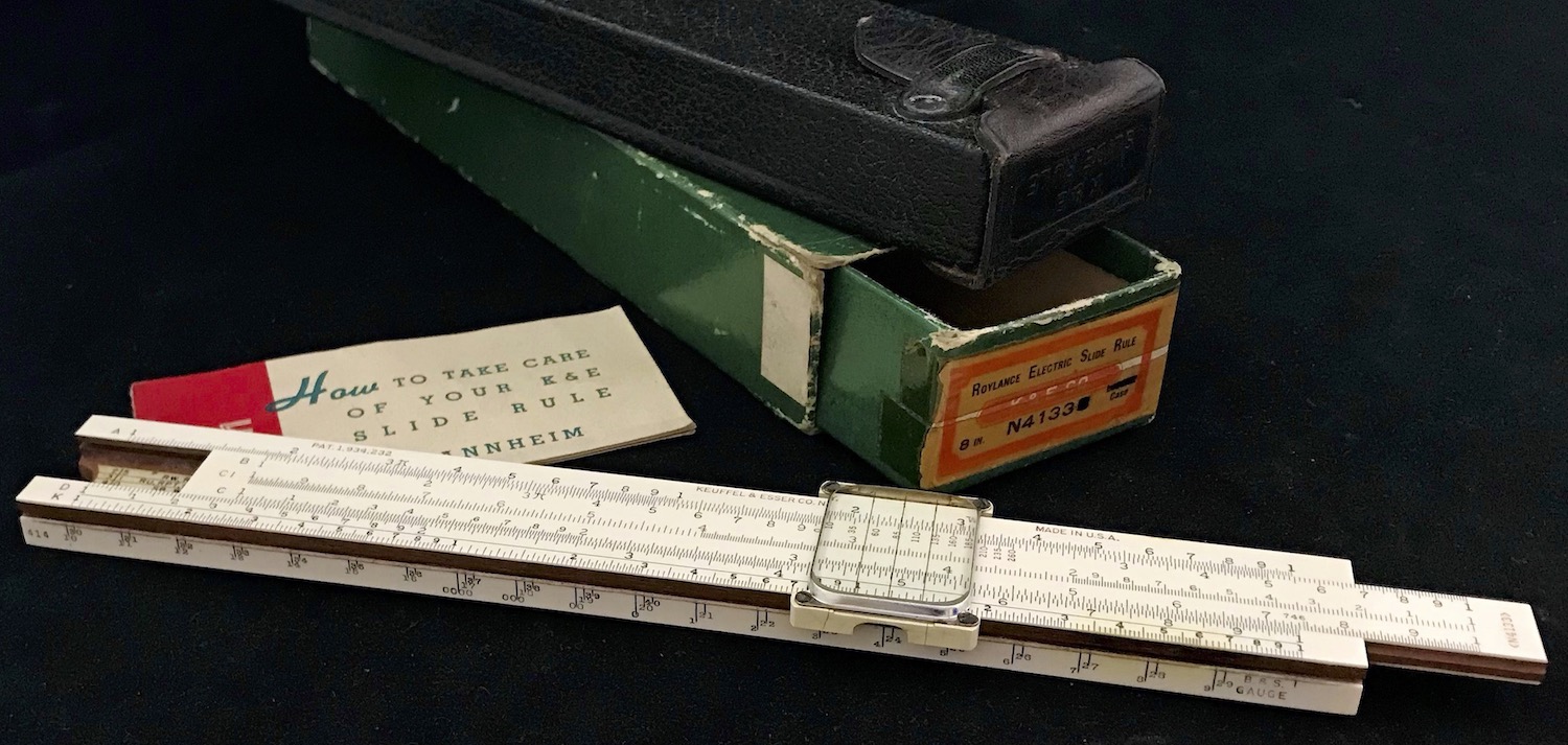
8.30.5 The Roylance Slide Rule
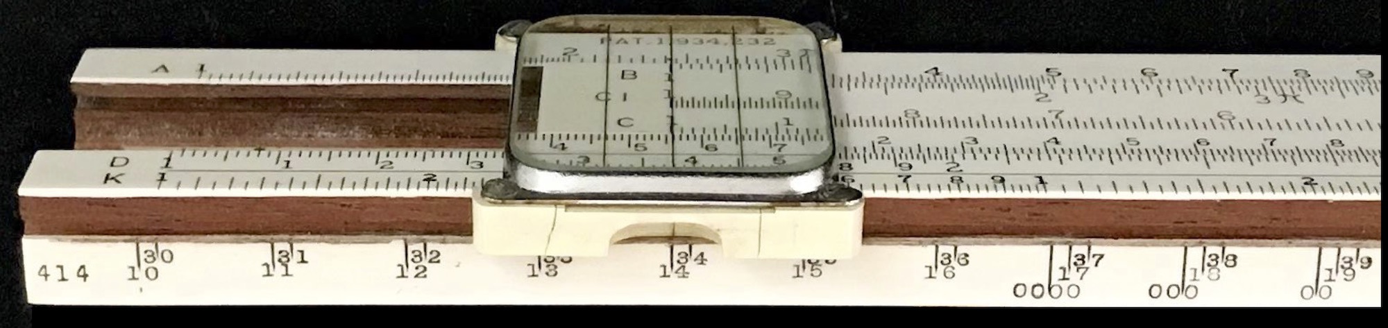
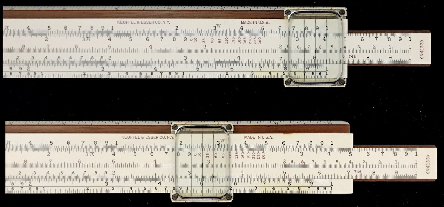
There is a variety of electro slide rules that have been made around the world which are either similar to the Faber-Castell 368, 378, 1/78 family of rules, or ones that provide similar scales and related gauge marks for performing electrical calculations. In the US, only one major maker produced an electrical slide rule – the 8-inch Keuffel and Esser Model 4133 Roylance Electrical Slide Rule. Created by Leon St. D. Roylance, of San Francisco, California, this slide rule design was made for use with the B&S/AWG gauge system. The Roylance was manufactured from 1913 to 1944, and the figure below shows the N4133 model from 1944. On the front face we see essentially the scale layout of the K&E 4053 Polyphase Mannheim slide rule, but with a small set of numbers, in red, overlaying a portion of the B scale. The cursor also has three hairlines, which is unusual for K&E rules. On the bottom edge are three rows of numbers, ranging from 0000 to 40, and labeled “B&S Gauge”. And the slide rule also has numbers inscribed in the well.
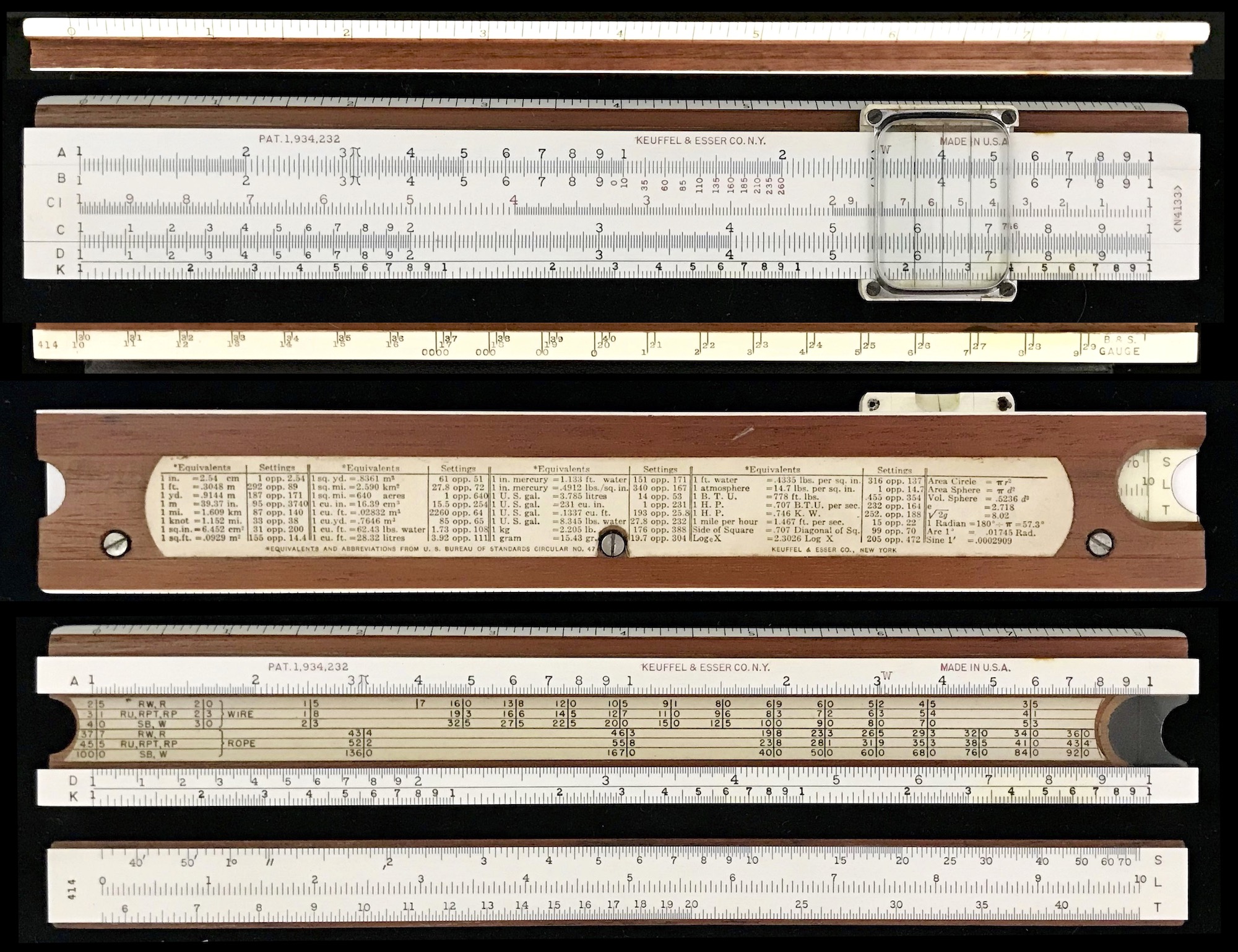
8.30.5.1 Gauge Parameters
As can be ascertained from the image, the Roylance Electrical Slide Rule was designed specifically for use with the AWG, or B&S, wire gauge system. The instructions that came with the rule tell the user to set the cursor on the lower edge of the rule to the gauge of the wire being used.
Then, move the index (usually the left index) to the cursor. Once this is set, several parameters can be read directly from the rule. For example, consider setting the slide rule as just described for AWG (B&S) gauge 14 wire; then, move the right-hairline on the cursor to the right index on D. Then,
- the wire diameter, in mils, is found on C above the right index on D – 64.1 mils.
- the cross-sectional area of the wire, in “circular mils”, is found on B under the right index on A – 4110 cmils.
- the cross-sectional area of the wire, in “square inches”, is found on B under the left hairline – 0.00323 in\(^2\).
- under the “W” Gauge Mark located on A, the weight in pounds of 1000 ft of wire will be found on B – 12.7 lbs.
A “circular mil”, by the way, is a unit of area, which in the early 1900s was given by the square of a diameter, in mils. Hence, a circle of diameter \(d\) has a value of \(d^2\) cmils; this is larger than the area of a circle of diameter \(d\) by a factor of \(4/\pi\) = 1.273 = 1/0.785.
If the right-hand hairline on the cursor is set to the index on D, then the cross-sectional area of the wire in “square inches” is found on B under the left-hand hairline. This is because the left- and right-hand cursor lines are separated, on the A/B scales, by the factor of \(4/\pi\) mentioned above, and 1 in\(^2\) = \(10^6\) mil\(^2\).
As can be imagined, one of the difficulties is to get the decimal point right for these readings. This takes practice and experience, and is described further in the instructions. Notice that the gauges listed on the bottom edge of the rule are written on three different lines:
- The first line starts with #0000 below about 2.15 on D, and goes to #9 near 10 on D.
- The second line starts with #10 near 1 on D and goes to #29 near 9 on D.
- The third line starts with #30 near 1 on D and goes to #40 near 3.2 on D.
Rather than employing a log-log scale to deal with the gauge diameters, Roylance took a slightly different approach. What we find is that the successive gauge marks on the bottom edge are displaced from each other by a distance that is given by our special ratio of \(1.1229\), as read on the C/D scales. They are marked so as to take readings on D, say, with successive decades. That is, since the bottom line goes with larger wires, then the numbers on C/D are taken to be from 100 to 1000 mils for those gauges. (Remember, #0000 is 460 mil diameter.) For gauges on the middle line, the numbers on C/D are treated as between 10 and 100. And for gauges found on the top line, the numbers on C/D are taken to be between 1 and 10. (For example, #36 has a 5 mil diameter.) The numbers on A/B are the squares, and so their decimal point locations can be inferred appropriately.
Since the B&S system deals only with one particular “base” in the exponential function for the wire diameter, where \(d \sim 0.89053^{AWG}\), the wire gauge can be marked along the edge of the slide rule using
\[ d \sim 0.89053^{AWG} ~~~~\longrightarrow ~~~~\log d \sim \log (0.89053)^{AWG} = AWG\cdot\log(0.89053) = -AWG\cdot\log(1.1229) \]
and hence a general log-log scale is not necessary.
Now since the resistance of the wire is inversely proportional to the square of the wire size – i.e., as the gauge number goes up, the size goes down and the resistance goes up – then as the gauge numbers go from left to right on the rule then their resistance can be read from left to right on the A/B scales, with an appropriate offset for the resistivity of copper. On the Roylance, if we move the cursor to one of the red numbers on B, and interpret that number as a temperature in Celsius, we can read off the resistance of 1000 feet of wire at that temperature on A. For the setting of our #14 wire, we find the resistance to be 2.53 Ohms at a temperature of 20 C. This can be seen in the bottom image of the figure above. For the middle line of wire gauges, the resistances are in the range of 1 to 10 Ohms; for the lower line, 0.1 to 1 Ohm (lower AWG, larger area, lower resistance); for the upper line, 10 to 100 Ohms – all per 1000 feet.
8.30.5.2 Voltage Drop and Other Parameters
Let’s compare the use of the Roylance to our previous example worked out using the FC 378 slide rule. Set the Roylance to align the index (right index, in this case) to the #4 gauge mark on the lower edge. For our case, the resistance at 20 C, say, will be about 0.25 Ohms. (Note that since we are on the lower edge scale, the resistance will be 1/10 that for gauges on the middle scale, etc.) This is for 1000 feet of wire. Our previous example was for 200 feet of wire (100 feet, back and forth). And so, for our example we should have a resistance of 0.05 Ohms; or a voltage drop rate of 0.05 V/A; or a voltage drop of 0.5 V for a current of 10 A – the same answer as before. But now, with the Roylance, we also can explore the variation of voltage drop with wire temperature.
Even more parameters of the chosen wire gauge can be found by placing the cursor at the proper wire gauge mark on the lower edge, and removing the slide. In the well of the rule will be a table for that gauge wire. Doing so for our #14 wire example, we find in the well under the cursor:
The meanings of the symbols are the following:
- “RW, R” are moisture resistant and code values.
- “RU, RPT, RP” are 90% unmilled grainless rubber, small diameter building wire, and performance conductors.
- “SB, W” are slow burning and weatherproof conductors.
The numbers, to be read as “15”, “18”, and “23” Amps, are the current-carrying capacities of the types of conductors for the given gauge. And the upper three lines found in the well are for bare wire, while the bottom three rows are for ropes made of wire (see the instructions). For our setting of the #14 wire, we see that to “meet code”, the current through this wire should not be allowed to exceed 15 A. Since our numerical example is using 10 A, then we’re all good.
8.30.5.3 Efficiency Calculations
Like most other electro rules, the Roylance includes a gauge mark on the C scale that allows for direct computation of dynamo and motor efficiencies. If the “746” gauge mark on C is set to the index on D, then any “HP” number on the D scale will be opposite its “KW” counterpart on the C scale. Thus, if a power reading in horsepower is known, its value in Watts can be readily found, and vice versa. With the same units for both input and output power, an efficiency ratio is then calculated using C/D.
We see that the Roylance slide rule provides a wealth of information to the user which can immediately be inserted into calculations on the spot. However, keeping track of units and decimal places is daunting. In the article by R. Hughes a number of tables help summarize many of the instructions for the Roylance slide rule, in terms of decimal points, L/R indexing, etc. This article is highly recommended for anyone interested in understanding all of the details about the use of this slide rule. I’m sure a bit of practice using the rule would help a great deal as well.
The electro slide rule is an elegant device that can be used to perform both general calculations and specialty calculations in the realm of the electrical trades. These rules are historically significant due to the need for them during the electrification of the world in the early 20th Century, and for their introduction of log-log scales into the mainstream of slide rule design. The slide rule collection presently contains a total of 10 electro rules which are summarized in the section Specialty Slide Rules.
Some nice references on the subject are:
- Bobby Feazel, “The Roylance Electrical Slide Rule”, Jour. Oughtred Soc. 6.2 p39 (1997).
- J.S. Pöll, “The Story of the Gauge”, Anaesthesia, 54 pp575–581 (1999).
- Robert Adams, “Elektro Rules: Their Use and Scales”, white paper from his presentation at IM2007. Available from The Oughtred Society.
- Richard Smith Hughes, “The Keuffel and Esser Roylance 4133 Electrical Slide Rule”, Jour. Oughtred Soc. 17.1 p42 (2008).
- Colin Tombeur and Trevor Catlow, “Early Faber Log-Log Scales”, Slide Rule Gazette, 20 p116 (2020).
- Electrical and Radio Slide Rule Instructions, International Slide Rule Museum Library Reprints - Volume 15, Amazon (2021).
Note that not all electo rules include this factor of two.↩︎
See J.S. Pöll, “The Story of the Gauge”, Anaesthesia, 54 pp575–581 (1999).↩︎
You might notice that the LL scales extend beyond the Left/Right indices on C/D and A/B. So long as the exponential operation stays on one scale or the other, all is well. But when the slide is set on the top LL scale, say, and the answer is on the bottom LL scale, then there is a problem. This is resolved using the “W” mark on the slide, just beyond 10 on C. At this point, I’ll just leave it at that, and refer the reader to the Tombeur and Catlow article listed at the end of this vignette.↩︎
See, for example, Robert Adams, “Elektro Rules: Their Use and Scales”, presentation, IM2007. Available from Oughtred Society.↩︎