8.42 Hemmi 153 Scales
Originally posted: 2021 Feb 08
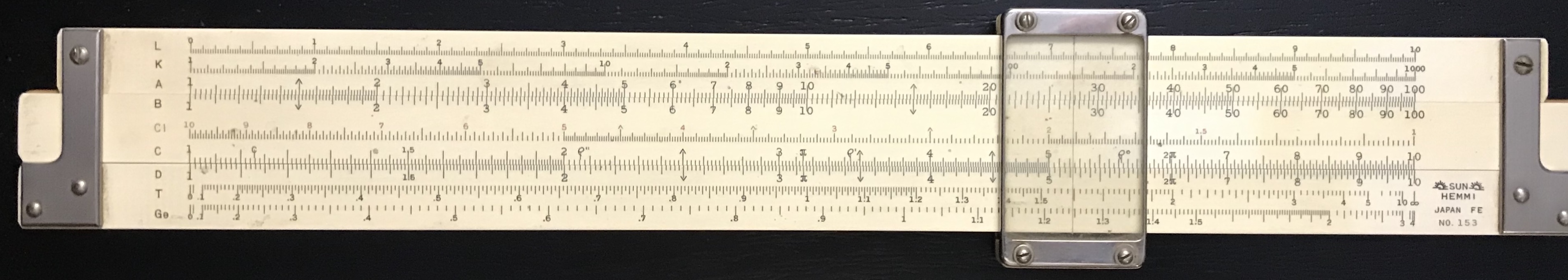
When the use of complex numbers in electrical engineering problems became more commonplace, vector slide rules were introduced by several manufacturers that made the evaluation of trigonometric functions with complex arguments much easier. The new rules had access to values of hyperbolic trigonometric functions which are needed to compute quantities such as the sine or tangent of a complex number. After such scales were introduced by K&E in the late 1920s, Hemmi (or, Sun Hemmi) came out with a new model – No. 153 Electrical Engineers Universal Duplex – which had its own unique set of scales for such problems.
A unique feature of the Model 153 was the central use of a mathematical function called the Gudermannian function167, which connects the circular trigonometric functions and hyperbolic functions without explicitly using complex numbers – exactly what was needed for the electrical engineering problems of the mid-20-th century.
The Gudermannian function, for real values of \(x\), can be defined in various equivalent ways as
\[\begin{eqnarray*} {\rm gd}~x &=& \int_0^x {\rm sech} u \; du \\ &=& \sin^{-1}[\tanh(x)] \\ &=& \tan^{-1}[\sinh(x)] \\ &=&2\tan^{-1}(e^{x}) - \frac{\pi}{2}. \end{eqnarray*}\]
A plot of the function is shown here:

Amazingly, this single function connects the exponential, trigonometric, and hyperbolic trigonometric functions without the use of complex numbers. From the above we see that the hyperbolic functions can be written in terms of trigonometric functions of the Gudermannian of \(x\):
\[ \sinh(x) = \tan({\rm gd}~x) ~~~~~~~~~~~~ \tanh(x) = \sin({\rm gd}~x) \] and the exponential function is given by \[ e^x = \frac{1+\sin({\rm gd}~x)}{\cos({\rm gd}~x)}. \]
So, on the Hemmi 153, while direct scales of hyperbolic functions are not present, their values can be found by taking the sine or tangent of values of the Gudermannian function. No doubt many may have felt that this was an over-complicated procedure, but others likely saw this as a very efficient and flexible arrangement of scales with far-reaching potential for use in a variety of mathematical problems.
\(~\)
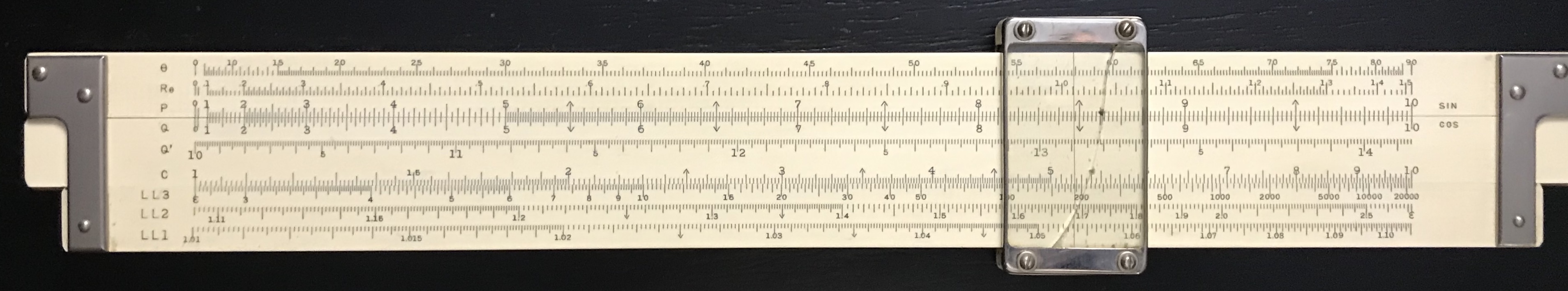
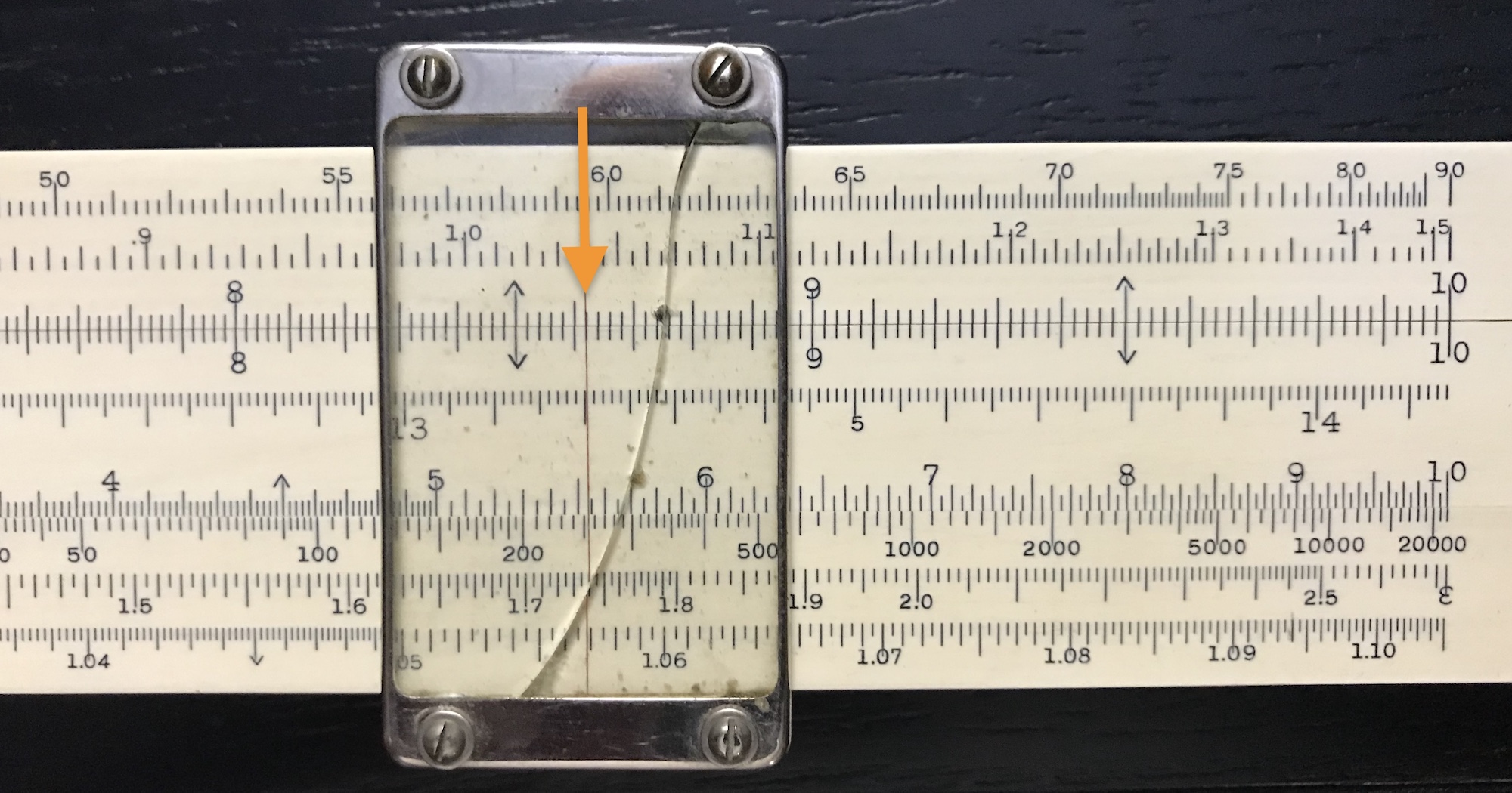
There were 18 basic scales on the Hemmi 153. Eleven of these are standard slide rule scales, namely L, K, A, B, CI, C and D on the front; and C, LL3, LL2, and LL1 on the back. It was the inclusion of seven new scales – none of which are logarithmic – which made the 153 stand out. Several of the new special scales eventually appeared on other Hemmi and Hemmi-inspired slide rules as well, but the Model 153 can be called a vector slide rule as it has access to the hyperbolic functions.
Following the discussion by Borchers and Cotter168, we can tie the new scales together through the L scale – which, on a standard slide rule, is actually a linear scale from 0 to 1. Let’s give a number on this scale a value \(0 \lt y \lt 1\). The P scale on the Hemmi 153 is not the P scale found on many other rules, particularly from Europe, which provides \(\sqrt{1-x^2}\). In the case of the Hemmi 153, its P scale gives the value of \(\sqrt{y}\), where \(y\) is on the L scale, and hence goes from 0 to 1. That is to say, the actual distance along the P scale from the left edge is proportional to the square of the number on the P scale. How is this useful? Well, it allows one to add the squares of numbers. So let’s add another identical scale – call it Q – to our rule. Then if we wanted to add \(3^2\) plus \(4^2\) we align the origin of the Q scale with the 3 on the P scale, find 4 on the Q scale and read off the answer “5” on the P scale – that is, the final distance along the scale is proportional to \(5^2\). We’ve just calculated \(\sqrt{P^2+Q^2}\).
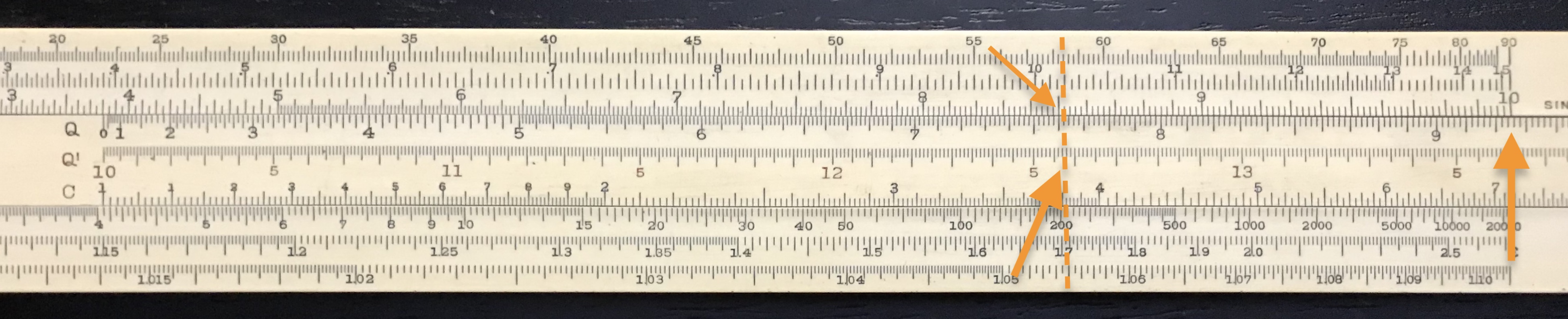
So what about the Q’ scale? As in the use of C/D scales, sometimes the answer falls off-scale. If we want \(\sqrt{0.8^2 + 0.9^2}\) we get 1.20 which is beyond 1.0. The Q’ scale gives \(\sqrt{1+y}\) and so extends the Q scale up to the value \(\sqrt{2}\). With the Q and Q’ scales, one can easily add numbers in quadrature or find quadratic differences. Here are a couple of examples:
- Example: Compute \(\sqrt{925^2 + 852^2}\): First of all, there’s an overall factor of 100 that temporarily can be taken out. That said, find 9.25 on the Q scale and align this with the right-hand-side of the P scale. Next, move the cursor to 8.52 on the P scale. The final answer will be read off of the Q’ scale (12.575) under the cursor line. Final answer: \(\times 100 = 1258\).
In addition to computing quantities like \(c=\sqrt{a^2 + b^2}\), we can also compute \(a=\sqrt{c^2 - b^2}\) by subtracting distances rather than adding them:
- Example: Compute \(\sqrt{9.25^2 - 8.52^2}\): Here, line up cursor with 9.25 on the P scale. Below, align 8.52 on the Q scale. The difference will be found on the P scale above the 0 on the Q scale: 3.60.
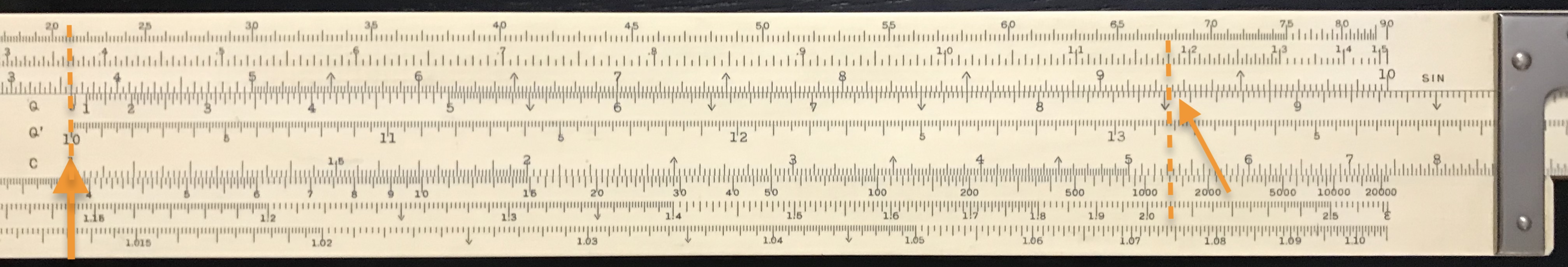
Given any two sides of a right triangle, one can directly compute the remaining side with the use of the P and Q/Q’ scales.
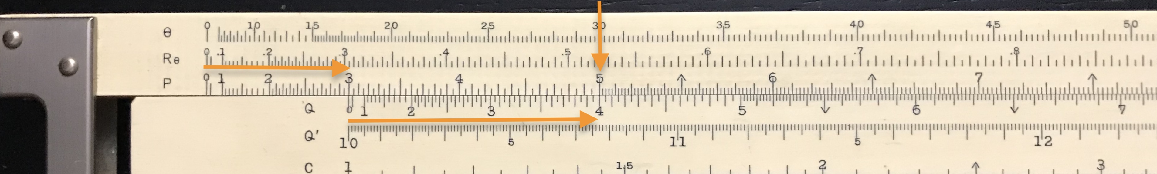
So we now have P and Q scales on the rule that each range from 0 to 1, and whose distances along the rule scale with the square of the numbers printed on the scales. Hemmi created the \(\theta\) scale to go from 0 to 90 deg such that the sine of the angle on the \(\theta\) scale can be read on the P scale. To find the cosine of the angle, one can just align one end of the Q scale with the angle in question and read the cosine at the end of the P scale, since \(\cos^2\theta + \sin^2\theta = 1\). Additionally, a separate angular scale for reading angles in radians was created: \(R_\theta\). Conversions between degrees and radians can be read directly from these two scales, plus trigonometric function values can be computed directly from either degree or radian numerical values.
- Example: Find \(\sin(0.83)\) – Since there is no “degree” symbol, the problem is referring to 0.83 radians. So, line up the cursor with 0.83 on the \(R_\theta\) scale. The sine of this angle is read directly on the P scale: 0.738.
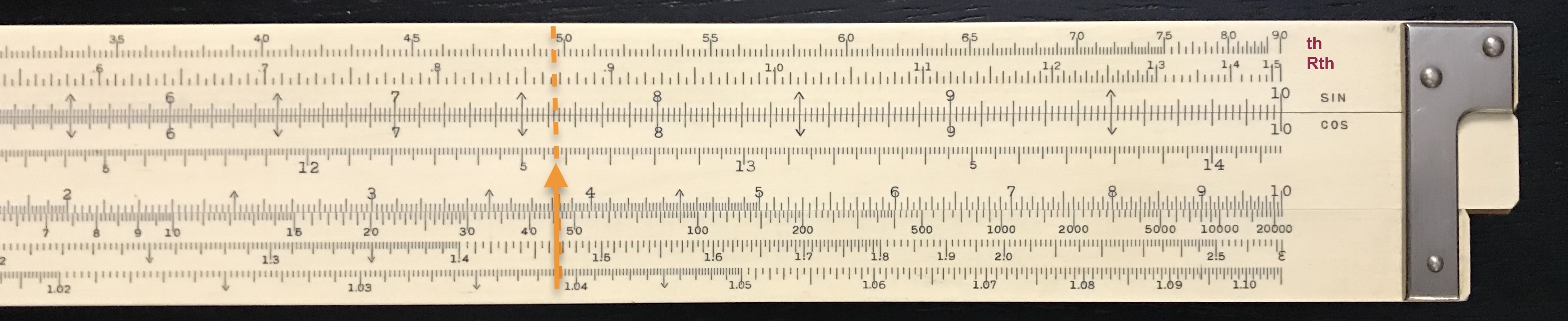
- Example: Find \(\cos(25^\circ)\) – Here, the cursor should become aligned with the 25 on the \(\theta\) scale. Line up the left edge of the Q scale with the cursor, and the cosine of the angle will be read at the right edge of the P scale: 0.906.
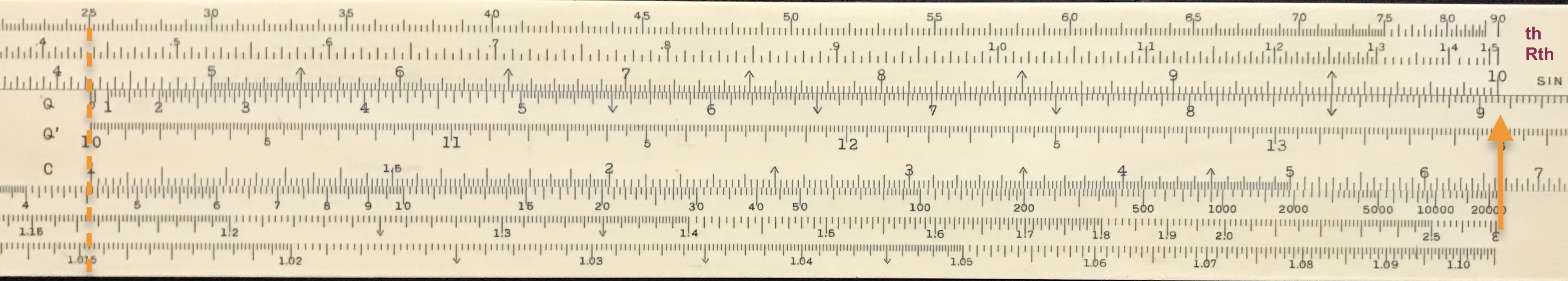
But now, a new scale for the tangent of an angle is necessary. This is found on the front of the Model 153. Unlike most T scales, this T scale gives the value of \(\tan x\) where \(x\) is on the \(\theta\) scale or \(R_\theta\) scale.
Finally, there’s the \(G_\theta\) scale, which is found at the bottom of the front side of the slide rule. This scale is essentially the inverse function \({\rm gd}^{-1}(x)\) and its purpose is to compute hyperbolic trig function values. In terms of our L scale which gives \(0 \lt y \lt 1\), the \(G_\theta\) scale goes like \(\tanh^{-1}(\sqrt{y})\). Since \(y\) is on the L scale and \(\sqrt{y}\) is on the P scale – which is the sine of the angle on the \(\theta\) or \(R_\theta\) scale – then a number on the \(G_\theta\) scale is the argument for which its hyperbolic tangent is found on the P scale. Voila!
Suppose we want the hyperbolic sine of an angle \(x\), which is provided in units of radians. As seen above, \[ \sinh(x) = \tan({\rm gd}~x). \] We locate the value \(x\) on the \(G_\theta\) scale and then, from the T scale, we read off the value of \(\sinh x\). Without moving the cursor, we can also flip the rule to directly read the value of \(\tanh x\) on the P scale, since \(\tanh(x) = \sin({\rm gd}~x)\). For example: \(\sinh 1.3 = 1.699\) and \(\tanh 1.3 = 0.862\).
The process may seem a bit contorted, but access to values of hyperbolic trigonometric functions using the Gudermannian function allows for vector calculations as described in section Vector/Hyperbolic Calculations to be performed with the 153. The unique scale set provides for a variety of vector-related calculations using a relatively small number of scales. The number of steps involved in evaluating functions of complex numbers using this rule, however, is often larger than the number required when using slide rules with direct hyperbolic scales tied to the logarithmic C/D scales.
Though the use of the Gudermannian function is rather unique to the Hemmi 153, other scales on this model – the P and Q scales in particular – have been adopted on other slide rules, such as the Lafayette Model F-686 and the Boykin Rota-Rule found in the Collection. (The Rota-Rule designates these scales as V1 and V2, but they perform the same calculation.) The F-686 is also a vector rule, but utilizes the standard hyperbolic function scales Sh and Th.
Below is a list of slide rules in the Collection that have the Hemmi-inspired P/Q scales:
| Maker | Model | Year | Fr Scale | Bk Scale |
|---|---|---|---|---|
| Hemmi | 153 | 1931-1934 | L K A [ B CI C ] D T Gtheta | theta Rtheta P [ Q Q’ C ] LL3 LL2 LL1 |
| Hemmi | 153 | 1936-1940 | L K A [ B CI C ] D T Gtheta | theta Rtheta P [ Q Q’ C ] LL3 LL2 LL1 |
| Hemmi | 153 | 1938 | L K A [ B CI C ] D T Gtheta | theta Rtheta P [ Q Q’ C ] LL3 LL2 LL1 |
| Hemmi | 153 | 1955 | L K A [ B CI C ] D T Gtheta | theta Rtheta P [ Q Q’ C ] LL3 LL2 LL1 |
| Relay-Ricoh | F-686 | 1961 | Tr1 Tr2 P’ P [ Q ST Sr Stheta C ] D LL01 LL02 LL03 | Sh1 Sh2 DF A [ B CF Th CI C _ LL1’ ] D LL3 LL2 db |
| Boykin | RotaRule Model 510 | 1965 | K A D [ C CI CF S CS ST T CT B L ] | D50 DLL V2 [ V1 C50 LL3 LL2 LL1 LL01 LL02 LL03 ] |
| Shanghai Slide Rule Factory | Flying Fish 1018 | 1975 | theta Rtheta P’ P [ Q QI L I ] J J’ T Gtheta | LL01 LL02 LL03 K A [ B T S C ] D DI LL3 LL2 LL1 |
Summary of Special Hemmi Scales on the Model 153:
| Scale | Use | Operation |
| L | standard linear scale | \(0\le y \le 1\) |
| \(\theta\) | angular measure (deg.) | \(\sin^{-1}(\sqrt{y})~~\) (deg.) |
| \(R_\theta\) | angular measure (rad.) | \(\sin^{-1}(\sqrt{y})~~\) (rad.) |
| \(G_\theta\) | Gudermannian function, \({\rm gd}(x) \equiv \sin^{-1}[\tanh(x)]\) | \(\tanh^{-1}(\sqrt{y})\) |
| \(P\) | sine of angular measure | \(\sqrt{y}\) |
| \(Q\) | sine of angular measure | \(\sqrt{y}\) |
| \(Q'\) | extended \(Q\) scale | \(\sqrt{1+y}\) |
| \(T\) | tangent of angular measure | \(\tan(\sin^{-1}(\sqrt{y}))\) |
Further Notes on the Gudermannian Function
Starting with the definitions \(e^x = \cosh x + \sinh x\) and \(e^{-x} = \cosh x - \sinh x\), we can define the hyperbolic functions in terms of a new function, call it \(G(x)\) for now, such that
\[ \tan G(x) \equiv \sinh x ~~~~~~ and ~~~~~~ \sin G(x) \equiv \tanh x. \]
Dividing the two, we see that \[ \cos G(x) = \frac{\sin G(x)}{\tan G(x)} = \frac{\tanh x}{\sinh x} = \frac{1}{\cosh x}. \]
Next, recall two basic trig identities:
\[ \tan(A+B) = \frac{ \tan A + \tan B}{1-\tan A \tan B} \]
and
\[ \tan(\frac{x}{2}) = \frac{\sin x}{1+\cos x}. \]
Putting this all together, one can find the Gudermannian function in terms of \(x\) in the following way, remembering that \(\tan (\pi/4) = 1\):
\[\begin{eqnarray*} \tan(\frac{G}{2}+\frac{\pi}{4}) &=& \frac{\tan(G/2) + 1}{1-\tan(G/2)} = \frac{\frac{\sin G}{1+\cos G}+1}{1-\frac{\sin G}{1+\cos G}} \\ &=& \frac{1+\cos G + \sin G}{1+\cos G - \sin G} = \frac{1+\cosh x + \sinh x}{1+\cosh x - \sinh x} \\ &=& \frac{1+e^x}{1+e^{-x}} = e^x\cdot\left\{ \frac{1+e^{-x}}{1+e^{-x}} \right\} \\ &=& e^x \end{eqnarray*}\]
Inverting things now, \(G/2 + \pi/4\) = \(\tan^{-1}(e^x)\), and so, as a general function of \(x\), the Gudermannian function is
\[ {\rm gd}~x = G(x) = 2\tan^{-1}(e^x)-\frac{\pi}{2}. \]
From calculus, the derivative of the tangent of \(x\) is \[ \frac{d}{dx}\tan x = \frac{1}{\cos^2 x} = \sec^2 x. \]
Using the chain rule and taking the derivative of both sides of the equation \(\tan(G/2 + \pi/4) = e^x\), we find that
\[ \frac{d}{dx}\tan(\frac{G}{2}+\frac{\pi}{4}) = \frac{1}{2}\sec^2(G/2 + \pi/4)\cdot\frac{dG}{dx} ~~~~ = ~~~~ \frac{d}{dx}e^x = e^x, \]
or,
\[
\frac{dG}{dx} = 2e^x\cos^2(G/2 + \pi/4) = 2\tan(\frac{G}{2}+\frac{\pi}{4})\cos^2(\frac{G}{2}+\frac{\pi}{4}) \\ = 2 \sin(\frac{G}{2}+\frac{\pi}{4})\cos(\frac{G}{2}+\frac{\pi}{4}) \\
= \sin(G+\frac{\pi}{2}) = \cos(G) \\
= \frac{1}{\cosh x}.
\]
Thus, the Gudermannian function also can be defined as
\[
{\rm gd}(x) = G(x) = \int_0^x \frac{du}{\cosh u} = \int_0^x {\rm sech}\; u\;\; du.
\]