8.41 Vector/Hyperbolic Calculations
Originally posted: 2022 Jun 20
Congratulations on making it to this section; and kudos if you make it to the end! Here we describe one of the more esoteric uses of a small collection of some of the mid-twentieth-century side rules. These so-called vector rules contain scales of the hyperbolic sine and hyperbolic tangent functions, typically noted by the symbols SH/TH, or Sh/Th. While the values of such functions can be useful in a variety of physics and engineering problems, the vector rules were particularly useful in electrical engineering where complex vector calculations were often performed routinely.
The phrase “complex vector calculation” does not refer simply to a “complicated” procedure; reference is to an operation on a specific type of object – a vector – that has two components (for the case of interest here). A complex number or a vector in the present context can be thought of as an ordered-pair of two numbers, such as a set of coordinates. On a map, moving to a point six miles away, 30 degrees North of East, can be represented as a vector. On the map, one might draw an arrow from the original point to the new point; the arrow has a length corresponding to 6 miles, and is pointed at an angle of 30\(^\circ\) north of due-east – two numbers are required to define the vector. Getting to this point would also be equivalent to moving 5.2 miles East and 3 miles North – again, two numbers are involved.

A similar “picture” appears when discussing complex numbers. A complex number is one that involves the square root of -1. Any real number when “squared” will give a positive result: \(2^2 = 4\); \((-2)^2 = 4\). A number that when squared yields a negative real number as a result is called an imaginary number. It can be imagined as a real number times the square root of -1. The symbol \(i\) (for imaginary) is used to denote \(\sqrt{-1}\), and so a real number \(y\) times i gives the imaginary number \(z = iy\). For example \((2i)^2\) = \(4\times i^2\) = \(4\times(-1)\) = \(-4\). Note that the imaginary number -2\(i\) also gives -4 when squared.
In engineering practice, the symbol \(j\) is often used rather than \(i\) but has the exact same meaning. The famous mathematician Leonhard Euler first used the symbol i in the 1700s to denote imaginary numbers. However, the symbol i is typically reserved to denote electrical current in engineering problems, and so j is substituted for i in many engineering textbooks.
In general, a complex number is defined as one with both real and imaginary parts. They can be written in the form \(z = x + iy\), where both \(x\) and \(y\) are themselves real numbers. As an example consider the square root of 8i. The square root of 8 is \(\sqrt{8}\) = \(2\sqrt{2}\) = 2.8284…, a real, although irrational, number. The square root of -8 will be 2.8284i. But what about \(\sqrt{8i}\)? It can be shown that \(\sqrt{8i}\) = \(2 +2i\). This can easily be checked by squaring this complex number:
\[ (2+2i)\cdot(2+2i) = 4 + 4i + 4i +4i^2 = 4 + 8i - 4 = 8i \] noting that \(i^2\) = -1.
8.41.1 Phasor Diagrams
Often times complex numbers are used in engineering and scientific problems related to oscillating systems, whereby one can denote an amplitude and a relative phase of the oscillation.
We are familiar with the standard trigonometric functions sine, cosine and tangent which were discussed in Trigonometric Scales. Combinations of these functions – the sine and cosine particularly – are solutions to systems which oscillate in time with constant amplitudes. For example, consider a vector like the one in our figure above. It has an amplitude (6 miles, in the example), call it \(r\), and a phase angle (30 degrees in our example), call it \(\theta\). Imagine that an object were to move along a circle of constant radius \(r\), with its angle \(\theta\) advancing at a constant rate, i.e., \(\theta = \omega \cdot t\). Though the length of the vector remains unchanged, it will rotate with time according to the advancement of the angle \(\theta\) = \(\omega t\), and the horizontal and vertical coordinates (\(x\) and \(y\)) on the map will oscillate according to
\[ x = r\cos\theta = r\cos\omega t, ~~~~~~~~~~~~ y = r\sin\theta = r\sin\omega t \]
as illustrated in the figure below.

Thus, the study of an oscillating system can be made equivalent to the study of a rotating vector. Note that the quantity \(\omega\) in the expression above is equal to \(2\pi\) times the oscillation frequency \(f\); when the time \(t\) becomes a multiple of the oscillation period \(T=1/f\), then the value of \(\omega t\) becomes a multiple of \(2\pi\) (= \(360^\circ\)) and the sine and cosine functions begin to repeat.
A complex number has two components, real and imaginary. By making a plot of the imaginary part vs. the real part and drawing it as an arrow (vector), we have an image of what is often referred to as a “phasor”. The phasor has an amplitude – the length of the arrow – and a phase angle (typically with respect the positive real axis). For example, the complex number we used above, \(2+2i\), can be drawn as a phasor as such:

In this example, the length of the phasor is \(r = \sqrt{8}\), while the phase angle has a value of \(\phi\) = 45 degrees (or, \(\pi/4\) radians).
8.41.2 Hyperbolic Trigonometric Functions
Oscillating systems are often analyzed in terms of rotating vectors or phasors. As shown above, a quantity oscillating at a fixed frequency, such as a particle on a spring or a current in an LC circuit, can be represented as a phasor. The mathematical solution for the equation describing such a simple harmonic oscillator (SHO) can be represented by the real component of a rotating vector, as described above. For systems in which oscillations are being driven by external sources or damped due to friction or resistance, for instance, then the solutions can involve amplitudes that grow or reduce exponentially. These solutions involve the so-called hyperbolic trigonometric functions:
\[ \sinh(u) = \frac{e^{u}-e^{-u}}{2}; ~~~~~~~ \cosh(u) = \frac{e^{u}+e^{-u}}{2} ; ~~~~~~~ \tanh(u) = \frac{e^{u}-e^{-u}}{e^{u}+e^{-u}}, \]
where the transcendental number \(e\) = 2.71828… is discussed in The Base of the Natural Logarithm. From these definitions we can describe exponential growth or decay in terms of these functions:
\[ e^{u} = \cosh u + \sinh u; ~~~~~~~~~ e^{-u} = \cosh u - \sinh u. \]
Below are graphs of the hyperbolic sine, cosine, and tangent functions:

These hyperbolic functions have a similar but slightly different set of “trig identities” as found among the standard trigonometric functions, but these will be left for the reader to discover elsewhere.
8.41.3 Connections to Standard Trigonometric Functions
The two sets of functions – standard trig functions and hyperbolic trig functions – can be connected by using complex numbers. In particular, standard trigonometric functions can be expressed in terms of the exponential function in an analogous fashion as for the hyperbolic trigonometric functions, if complex numbers are used:
\[ \sin\theta = \frac{e^{i\theta}-e^{-i\theta}}{2i}; ~~~~~~~ \cos\theta = \frac{e^{i\theta}+e^{-i\theta}}{2}; ~~~~~~~ \tan\theta = -i\;\frac{e^{i\theta}-e^{-i\theta}}{e^{i\theta}+e^{-i\theta}}. \] Taking the first two relationships above and solving for \(e^{i\theta}\),
\[ e^{i\theta} = \cos \theta + i\sin \theta. \]
This identity, that connects the exponential function (and, hence, the natural logarithm, with \(e\) as its base) with the two trigonometric functions sine and cosine through the imaginary number \(i = \sqrt{-1}\), is known as Euler’s Formula, after the famous mathematician Leonhard Euler.165
Taking this result and multiplying through by a “radius” \(r\),
\[ re^{i\theta} = r\cos \theta + i(r\sin \theta) \equiv x + iy. \]
The notion of a vector appears. Thinking of the complex number as an arrow in a 2-dimensional plane, then its purely “real” component is in the \(x\) direction and its purely “imaginary” component is in the \(y\) (or \(iy\)) direction. The above relationship shows that \(x = r\cos\theta\) and \(y=r\sin\theta\). The values \(x\) and \(y\) are the Cartesian coordinates of the vector \(z = re^{i\theta}\) in the complex plane, as shown here:

8.41.4 Multiplication of Complex Numbers
Given the amplitude and phase angle \(r\) and \(\theta\) of the complex number \(z = re^{i\theta}\), we can compute its real and imaginary parts using \(x=r\cos\theta\) and \(y=r\sin\theta\). Likewise, given \(x\) and \(y\), one can find the phase angle and the amplitude: \(\theta = \tan^{-1}(y/x)\) and \(r = \sqrt{x^2 + y^2} = y/\sin\theta\). Performing such calculations on standard slide rules with trigonometric scales were common. And the addition of two complex numbers is straightforward enough: just add the two real portions to get the real portion of the result, and then do the same for the complex portions.
On the other hand, computing the product of two complex numbers is somewhat simpler when written in polar notation. For instance, to find the product of two complex numbers \(z_1\) and \(z_2\), we could
write each complex number in Cartesian coordinates such as \(z_1 = x_1 + i y_1\) and \(z_2 = x_2 + i y_2\), from which the product would be \[ z_1z_2 = (x_1 + i y_1)\cdot(x_2 + i y_2) = x_1x_2-y_1y_2 + i(x_1y_2+y_1x_2) \] or, equivalently, we could
write each complex number in polar coordinates such as \(z_1=r_1e^{i\theta_1}\) and \(z_2=r_2e^{i\theta_2}\), from which the product would be \[ z_1z_2 = r_1r_2 \;e^{i(\theta_1+\theta_2)}. \] With the numbers given in polar notation, one just multiplies the two amplitudes and then add up the phases.
Some slide rules were advertised to be vector rules due to the fact that they allowed for easy conversions between Cartesian and polar coordinate systems, or allowed for more straightforward computations of the sides or hypotenuse of a right triangle. However, these operations do not involve hyperbolic functions. It was for the more-direct calculation of trigonometric functions of complex variables that brought about the invention of the true vector slide rule, as will be discussed next.
8.41.5 Functions of Complex Numbers
The result of applying a trigonometric function to a real number will be another real number. The sine of \(\pi/6\) (a real number, equivalent to \(30^\circ\)) is 0.5 (a real number). On the other hand, applying a trig function to a complex number in general will result in another complex number. For example, the sine of a purely imaginary number can be computed as follows:
\[ \sin(iy) = \frac{e^{i\times iy}-e^{-i\times iy}}{2i} = \frac{e^{-y}-e^{y}}{2i} = -\frac{e^{y}-e^{-y}}{2i} = i\sinh y. \]
That is to say, given an imaginary number \(iy\), finding the sine of this quantity results in a new imaginary number, namely \(i\) times the hyperbolic sine of the real number \(y\). In similar fashion one finds \(\cos(iy) = \cosh y\) (a real number in this case), and \(\tan(iy) = i\tanh y\) (a new imaginary number).
The sine of a general complex number \(z_0=x_0+iy_0\) is computed in a similar way:
\[\begin{eqnarray*} \sin z_0 &=&\sin(x_0+iy_0) = \frac{e^{ix_0-y_0}-e^{-ix_0+y_0}}{2i} = \frac{e^{ix_0}e^{-y_0}-e^{-ix_0}e^{y_0}}{2i} \\ &=& \frac{(\cos x_0+i\sin x_0)e^{-y_0}-(\cos x_0-i\sin x_0)e^{y_0}}{2i} \\ &=& \frac{-(e^{y_0}-e^{-y_0})\cos x_0 +i\sin x_0(e^{y_0}+e^{-y_0})}{2i}\\ &=& \sin x_0 \cosh y_0 +i \cos x_0 \sinh y_0. \end{eqnarray*}\]
So given a complex number \(z_0 = x_0 + i y_0\), taking the sine of \(z_0\) will yield a new complex number \(z\) given by
\[ z = x + iy = \sin z_0 = \sin x_0 \cosh y_0 +i \cos x_0 \sinh y_0. \]
By having access to tables or scales of standard hyperbolic trig functions, one can readily compute complex values of trig functions for complex arguments. This was the initial impetus for the design of the vector slide rules with scales of hyperbolic trig functions.
As another example, the hyperbolic sine of our general complex number \(z_0\) can be found as follows:
\[\begin{eqnarray*} \sinh z_0 &=& \sinh (x_0+iy_0) = \frac{e^{x_0+iy_0}-e^{-x_0-iy_0}}{2} = \frac{e^{x_0}e^{iy_0}-e^{-x_0}e^{-iy_0}}{2} \\ &=& \frac{e^{x_0}(\cos y_0+i\sin y_0)-e^{-x_0}(\cos y_0-i\sin y_0)}{2} \\ &=& \frac{(e^{x_0}-e^{-x_0})\cos y_0+i(e^{x_0}+e^{-x_0})\sin y_0}{2} \\ &=& \sinh x_0\cos y_0 + i\cosh x_0\sin y_0 \end{eqnarray*}\]
or,
\[ z = x + iy = \sinh z_0 = \sinh x_0\cos y_0 + i\cosh x_0\sin y_0. \]
Again, the result involves products of standard trig functions and hyperbolic trig functions. Naturally, similar expressions can be found for the functions \(\cos\), \(\cosh\), \(\tan\), and \(\tanh\) as well. Here is a table of the results:
| If \(~~z\) | = | \(x+iy,~~~~\) then … |
| \(\sin(z)\) | = | \(\sin x \cosh y + i \cos x \sinh y\) |
| \(\cos(z)\) | = | \(\cos x \cosh y - i \sin x \sinh y\) |
| \(\tan(z)\) | = | \((\sin 2x+ i \sinh 2y) / (\cos 2x + \cosh 2y)\) |
| \(\sinh(z)\) | = | \(\sinh x \cos y + i \cosh x \sin y\) |
| \(\cosh(z)\) | = | \(\cosh x \cos y + i \sinh x \sin y\) |
| \(\tanh(z)\) | = | \((\sinh 2x + i \sin 2y) / (\cosh 2x + \cos 2y)\) |
To get a better grip on the type of computations being discussed, a computer calculation can be performed. Using the computing language R, variables with complex values can be defined and values of functions of these variables can be computed. For example,
# Define value of z0 (a complex number):
z0 = 1.0+1.5i
# Find the sine of this number directly:
sin(z0)
## [1] 1.979484+1.150455i# Now, perform the calculation in steps...
# Select the Real, Complex components of the original z0:
x0 = Re(z0)
y0 = Im(z0)
# Individually Compute and Compare the
# Real and Complex components of sin(z0):
sin(x0)*cosh(y0)## [1] 1.979484## [1] 1.150455Here is a plot of the calculation just performed:

If a complex number \(z\) is recognized in terms of a vector, applying a function like \(\sin z\) or \(\cosh z\) will produce a new vector, with perhaps a new amplitude and phase angle. With hyperbolic trig scales on the slide rule, and appropriately placed regular trigonometric scales, the components of the results of complex vector calculations can be performed expediently on the rule.
For fun, a plot of \(\sinh z\) for a small collection of complex values \(z\) is created below. Here, the initial \((x_0,y_0)\) (“o”’s) and final \((x,y)\) (“+”’s) points in the complex plane are plotted, rather than drawing arrows from the origin:
8.41.6 A Vector Calculation on a Slide Rule
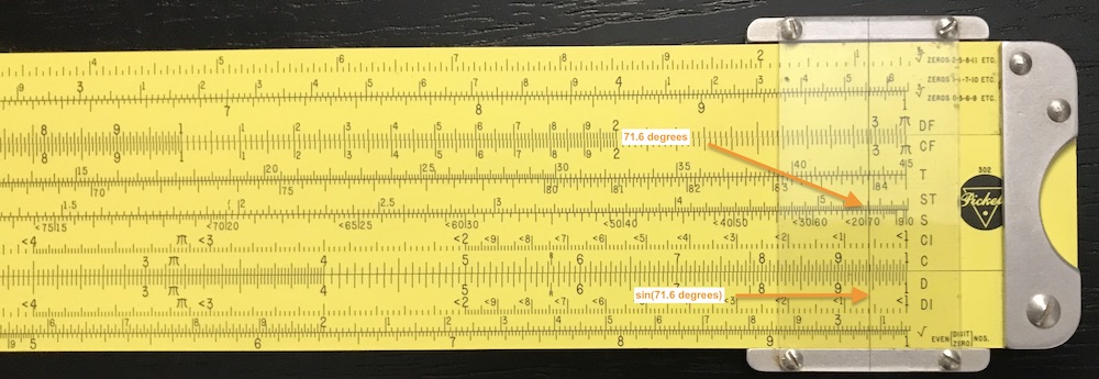
Taking one of the points in the plot above, the calculation of \(\sinh z_0\) is now performed on a slide rule. To illustrate, the Pickett Model 4-ES is used for our calculation. Suppose \(z_0 = 1 + 1.25i\). The desired result is \(z = \sinh z_0 = \sinh 1\cos 1.25 + i\cosh 1\sin 1.25\). Most rules, including the one used here, express the arguments of the standard trig functions in units of degrees rather than radians, and so the \(\sin\) and \(\cos\) arguments above must be converted accordingly. On the 4-ES there is a Gauge Mark “R” at 5.73 on the C/D scales – 57.3 degrees per radian – so this feature is used.
The problem is set up as follows. To get the real component of the final vector, compute
\[ \sinh 1\cos 1.25 = \sinh 1 \times \cos (1.25 \times 57.3^\circ ) \]
To perform the calculation here are the steps that I used:
- Line up the cursor on 1.25; line up the “1” under the cursor; slide cursor to the R gauge mark; read off degrees (= 71.6);
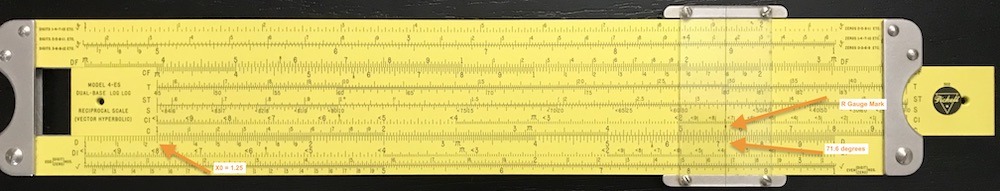
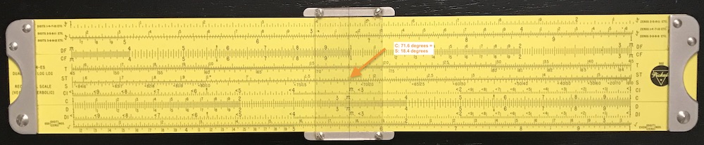
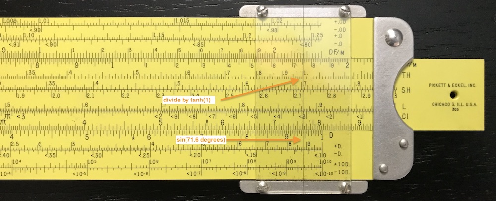
- Reset the slide; read cos(71.6) = 0.315 using cursor;
- Align left side of slide w/ cursor; move cursor to SH of 1.0;
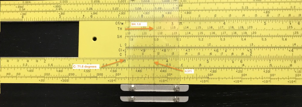
Read answer on D scale: 3.71
Think about the numbers a moment to realize that it is actually 0.371: \(~~~ x = {\rm Re}(z) =\) 0.371.
Next, to get the imaginary component of the final vector, we use
\[ \cosh 1\sin 1.25 = \sinh 1/\tanh 1 \times \sin (1.25 \times 57.3^\circ ) \] and the steps I used are:
- Reset the slide; align cursor to sin(71.6) = 0.95;
- Align TH 1.0 w/ cursor
- Move cursor to SH of 1.0;
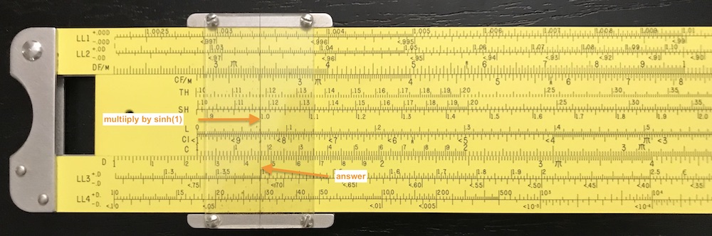
Read answer on D scale: 1.46
Think about the numbers a moment to realize that it actually is 1.46: \(~~~y = {\rm Im}(z) =\) 1.46.
Hence, the final answer is: \(~~\sinh(1+ 1.25i)\) = \(0.371+1.46i\).
\(~\)
Compare with a computer-generated calculation:
## [1] 0.3705672+1.46436iNow imagine making our last plot above with 17 total evaluations using a slide rule, compared to using our modern laptop computers!
8.41.7 Trig in Polar Coordinates
The result of taking vector \(z\) and performing a trigonometric function on \(z\) yields a new vector – essentially it takes the vector and rotates it, but it also can affect its length. On some vector slide rules, the layout of the appropriate scales on the stock and slide of the rule allow for more direct conversions from the polar coordinates (\(r\), \(\theta\)) of the first vector to the polar coordinates of the final vector. This was an invention of Mendell Weinbach, USA, in the late 1920s, which was first implemented on the K&E Model 4093-3 – the first vector slide rule – as well as on their later Models 4083-3 and 4083-5.166 Other manufacturers soon followed with their own models of vector rules.
Earlier it was shown that if \(z_0 = x_0 + iy_0\) then \(\sinh z_0\) = \(\sinh x_0 \cos y_0 + i \cosh x_0 \sin y_0\). If polar notation is used, where \(z=x+iy\) = \(re^{i\theta}\), then the new vector \(re^{i\theta}\) = \(\sinh( r_0e^{i\theta_0} )\) can be found in the following way. First, the final angle \(\theta\) can be found from the two Cartesian coordinates of the original vector: \[ \tan\theta = y/x = (\cosh x_0 \sin y_0)/(\sinh x_0 \cos y_0 ) = \tan y_0/\tanh x_0. \] Then, knowing \(\theta\), the final amplitude \(r\) can be solved for accordingly:
\[\begin{eqnarray*} r^2 &=& \sinh^2 x_0 \cos^2 y_0 + \cosh^2x_0\sin^2y_0 \\ &=& \sinh^2 x_0 \cos^2 y_0\left[1+(\cosh^2x_0/\sinh^2x_0)(\sin^2y_0/\cos^2y_0)\right] \\ &=& \sinh^2 x_0 \cos^2 y_0\left[1+\tan^2y_0/\tanh^2x_0\right] = \sinh^2x_0\cos^2y_0(1+\tan^2\theta) \\ &=& \sinh^2x_0\cos^2y_0/\cos^2\theta, \end{eqnarray*}\]
or,
\[ r = \sinh x_0\cos y_0/\cos \theta. \]
To summarize this current example, given an initial complex number \(z_0 = r_0e^{i\theta_0}\), the hyperbolic sine of \(z_0\) is computed through the following steps. First, find the real and imaginary Cartesian coordinates for this vector,
\[\begin{eqnarray*} x_0 &=& r_0 \cos\theta_0 \\ y_0 &=& r_0 \sin\theta_0 \end{eqnarray*}\]
and then find the \((r,\theta)\) components of the vector \(\sinh z_0 = re^{i\theta}\) using
\[\begin{eqnarray*} \theta &=& \tan^{-1}(\tan y_0/\tanh x_0), {\rm ~~ and~then} \\ r &=& \sinh x_0\cos y_0/\cos \theta. \end{eqnarray*}\]
Without hyperbolic scales on the slide rule, every \(\sinh x\), \(\cosh x\), and \(\tanh x\) operation above would require looking up values of \(e^x\) and \(e^{-x}\) and writing down results and forming various combinations. Having hyperbolic scales and the standard trig scales on the slide of a duplex slide rule can often greatly reduce the number of steps in the calculation. Similar methods and steps can be followed to compute other trig and hyperbolic trig functions of complex numbers as were performed above. To do so in an optimal way with a particular rule, one may need the instructions that came with it.
A slide rule with appropriately placed hyperbolic and standard trigonometric scales can readily compute trig and hyperbolic trig functions of complex numbers in a relatively small number of steps. Prior to these Vector rules, computing such numbers from tables and standard slide rules could take many times longer than could be done with the newer slide rules incorporating scales of the hyperbolic trig functions.
For a complete list of vector slide rules in the Collection, see Vector Hyperbolic Rules.
Euler’s Formula can be found in many textbooks on mathematics, physics, and engineering. See, for example, Mary L. Boas, Mathematical Methods in the Physical Sciences, John Wiley & Sons, New York, p. 60 (1983).↩︎
M.P Weinbach and A.F. Puchstein, The Log Log Vector Slide Rule, Keuffel and Esser Co., New York (1930).↩︎