8.35 Following the Balloons
Originally posted: 2023 Aug 11
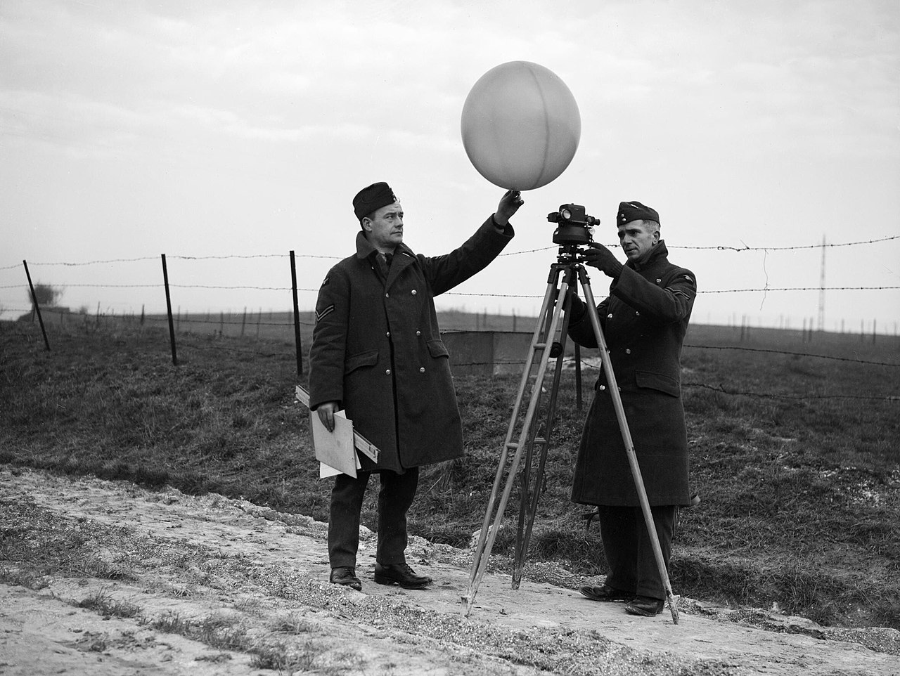
Since the systematic development of aviation in the early 20th century, balloons have been used by the world’s military and meteorological communities to ascertain the wind speed and direction at various altitudes in the earth’s atmosphere. Since the early 1900s the typical technique was to send up what was called a “pilot balloon” which had a “tail” of known length attached to it. As the balloon rose and drifted across the sky, tachyometric telescopes or theodolites (similar to those used in stadia measurements) would measure the angle from the ground to the balloon, and measure the visual angular extent of the tail hanging below the balloon.
 |
 |
|
| An early weather balloon launch. (Photo courtesy The History of Weather Balloon.) | RAF corporals with balloon and theodolite in 1940 England. Notice the large slide rule held by the man on the left. (Photo courtesy Air Ministry Second World War Official Collection.) |
By repeating such measurements from different ground stations at regular time intervals and triangulating, the ground coordinates and altitude of the balloon could be ascertained as well as its velocity. While such trigonometric calculations could in principle be performed using a standard slide rule, special slide rules were developed in England beginning in 1915. When the analysis was being repeated in the field every minute or so, a special slide rule would certainly be advantageous.
The geometry of the problem is depicted in the following figure.
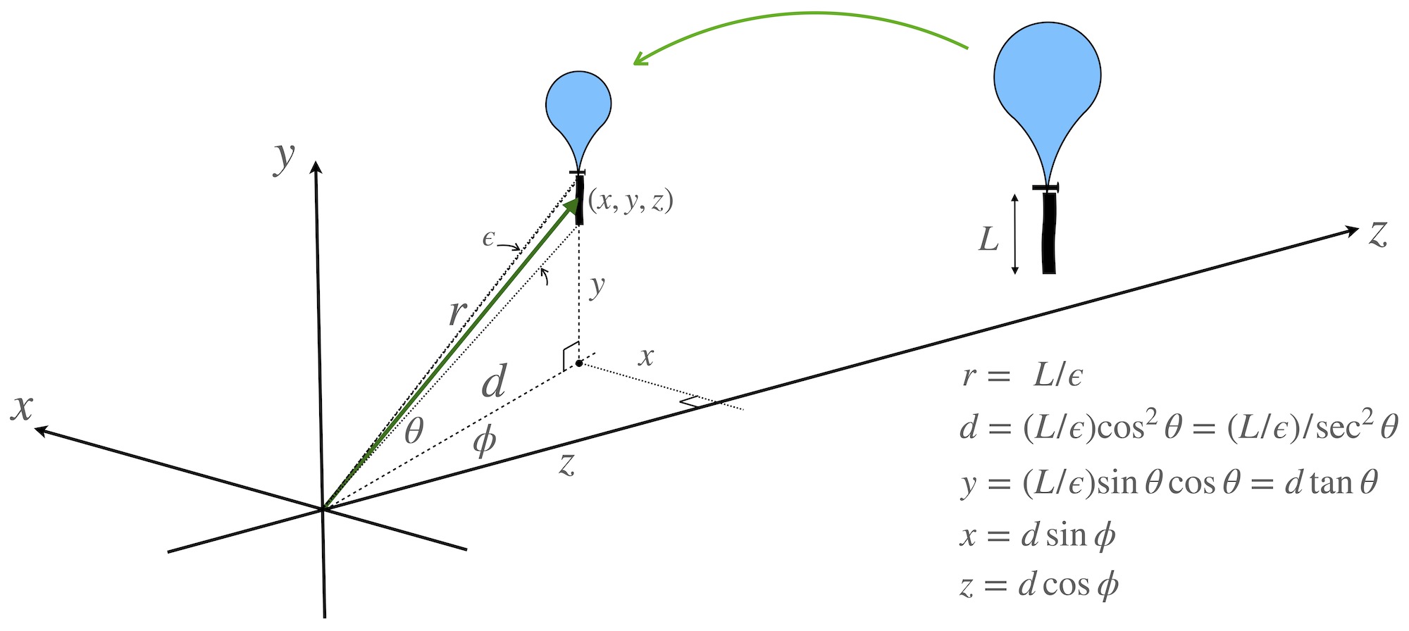
In the sketch above, the first three equations come from our stadia discussion. Here, \(L\) is the length of the tail hanging from the bottom of the balloon. A typical length was about 120 feet. The telescope used would have graticule lines that are visible through the eyepiece and measure angular field of view. Suppose there are \(k\) graticule lines per radian of angular view. If when viewed through the telescope the tail subtends m graticule lines, then the distance to the balloon is
\[ r = L/\epsilon = L\times k/m \equiv C/m. \]
A common value of \(C = L\;k\) would have been 120 feet \(\times\) 1000 = \(12\times 10^4\) feet.148 So, for example, if the tail subtends \(m\) = 60 lines in the eyepiece, the balloon would be 2000 feet away; if \(m\) = 10 then the balloon is 12000 feet away, and so forth.
From the equations for the coordinates we can see that if we solve for \(d\) in each case, then
\[ d ~~~~~~=~~~~~~ \frac{x}{\sin\phi} = \frac{z}{\cos\phi} = \frac{y}{\tan\theta} = \frac{L/\epsilon}{\sec^2\theta} . \]
Slide rules were designed to create the simultaneous ratios shown above. The measurement and calculation would go something like this:
- Using a transit telescope with graticule divisions visible through the eyepiece, measure the angular field of view \(\epsilon = m/k\) that subtends the upper and lower edges of the flag of known length \(L\).
- Also from the transit telescope, record the angles \(\theta\) and \(\phi\) that aim the telescope at the flag.
- Set the slide of the slide rule to place \(L/\epsilon\) against the value of \(\theta\) on the \(\sec^2\theta\) scale.
- Against the values of \(\phi\) and \(\theta\), read off values of \(x\), \(y\), and \(z\) on the appropriate trigonometric scales.
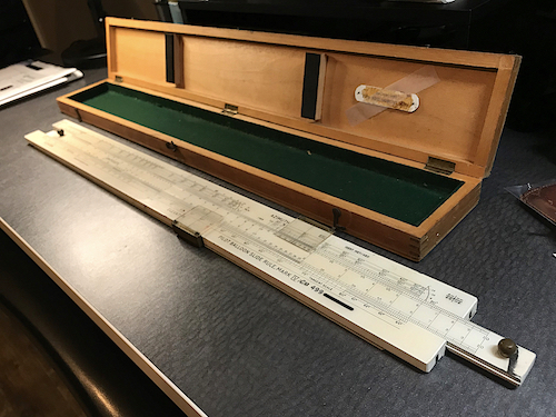
Pilot balloon slide rules were first introduced in 1915 for use of the Meteorological Office in England.149 The first model, the Mark I, was made of laminated wood and had two slides and three cursors. For the Mark II, which seems to have been introduced in about 1927, only one slide was needed, though a fourth cursor was added. The models continued to evolve, leading to the Mark III, Mark IV, Mark IV-A, Mark V, and the Mark 5 which was introduced in 1970. Throughout this evolution the basic computational process did not change appreciably. The Mark V was advertised in a London office supply catalog in 1974 for a price of £140.150 Naturally, by the late 1970s electronic calculators replaced the use of these slide rules in the field. As these devices were only for use by government agencies and relatively few were made, the Pilot Balloon slide rules are fairly rare.
Below is an image of the Mark IV-A slide rule in the Collection. This slide rule came to me from the Melbourne region of Australia.151 It is missing two of its four cursors, and appears to have seen a lot of action in its years of service. This slide rule, which is 24.5 inches long, was manufactured by Blundell Rules Limited in the United Kingdom, sometime between about 1957 and 1964, as estimated from other known examples. The scales are designed to be used with a flag/theodolite system with \(C=Lk = 1.2\times 10^5\) feet.
Let’s do an example calculation using the slide rule. Suppose a transit telescope is set up such that \(\phi\) = 0 corresponds to due east. Our balloon is traveling generally toward the northeast. In our coordinate system, positive \(x\) corresponds to north, positive \(z\) corresponds to east. Suppose the telescope is aimed at the flag of the balloon and a measurement is made in which \(\theta\) = 35 degrees, \(\phi\) = 17 degrees. The length of the tail as viewed in the telescope extends across \(m\) = 22 graticule lines. The tail of the flag on the pilot balloon is 120 feet long, and the view in the telescope contains \(k\) = 1000 graticule lines per radian.
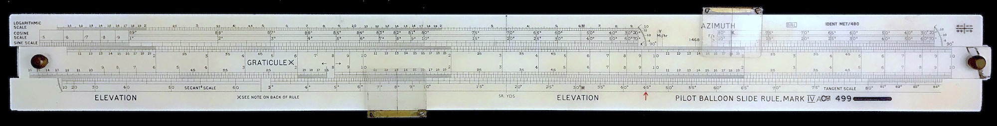
The slide is set by using the Graticule scale on the left side of the slide, and the Secant\(^2\) scale located on the bottom of the stock. The two scales (Secant\(^2\) on the left and Tangent on the right) on the bottom are for the elevation angle (\(\theta\)). From the measurement, we set 22 on the Graticule scale against an angle of 35 deg. on the Secant\(^2\) scale, as shown below.
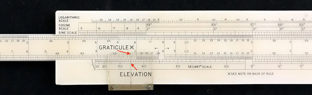
The slide rule is now set for the other calculations. For instance, if we move a bottom cursor over to the same angle of 35 degrees on the Tangent scale, we can read off the elevation of the balloon – we get a value for \(y\) of about 2570 feet.
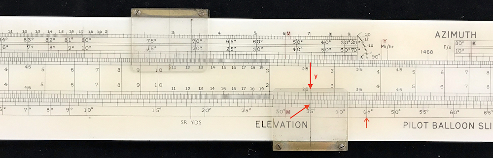
The angle scales on the top of the stock are for the azimuthal angle, \(\phi\). The upper angular scales are for \(\cos\phi\), and the lower angular scales are for \(\sin\phi\).
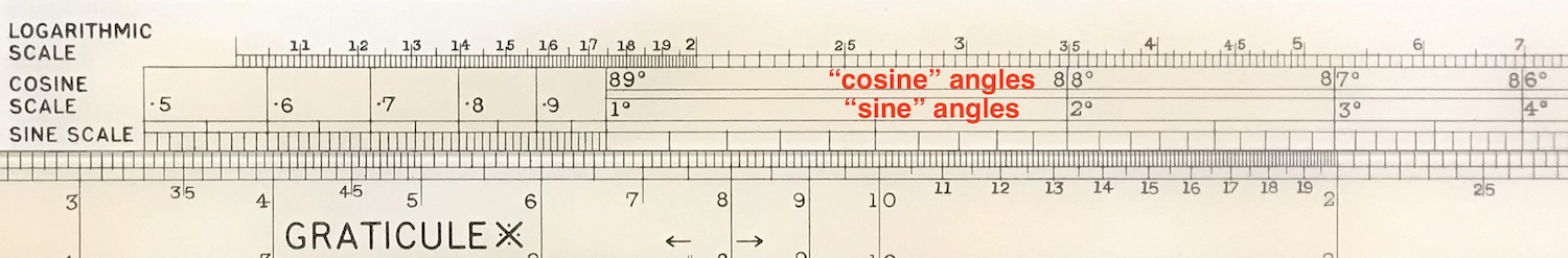
So, moving a cursor over to a value of 17 degrees on the “sine scale” we can read off the value for \(x\) on the slide; we get a value of about 1070 feet.
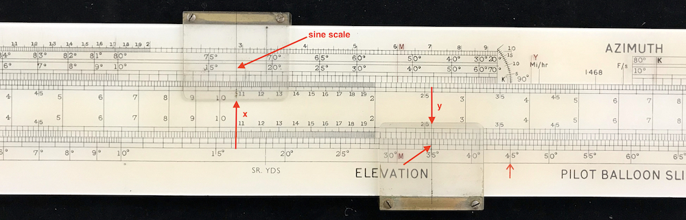
Moving the slide to the value of 17 degrees on the “cosine scale” we find the value of \(z\) on the slide; we see \(z\) is about 3500 feet.
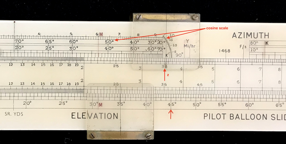
Note that as the angle \(\phi\) gets smaller, the lines on the cosine scale get closer together. The “arc” at the right end of the scale allows one to more easily set the cursor on small angles. It is on this arc that we set the cursor to the “17 degrees” mark.
The slide rule gives very accurate results. Using the computer we get for our measurement numbers, \(x\) = 1070, \(y\) = 2563, and \(z\) = 3500.
In general, the slide can be thought of as a single 3-decade logarithmic scale 22.5 inches long (7.5 inches per decade) from 1 to 1000 (or 10 to 10,000, etc.). The upper scale on the slide is indeed just this. The lower scale on the slide is a duplicate of the upper scale, except that it is interrupted on the left end to provide space for the “Graticule” scale. The values along the various trigonometric scales evolve in correspondence with this 7.5 inch decade spacing.
At the top left of the stock of the slide rule is a 2-decade logarithmic scale 15 inches long, again 7.5 inches per decade. Thus, it can be used against the upper scale on the slide to perform standard multiplication and division calculations.
Meteorologists would launch balloons and follow their journey often with a series of theodolites, taking measurements at regular time intervals. By recording data every two minutes or so, the assistant using the slide rule could create a table or plot of the data as the measurements went on. With this information, the meteorologists could plot out not only the location of the balloon but also its speed – and hence the local wind velocity – as a function of altitude and location.
See, for example, F. J. W. Whipple, “The Pilot Balloon Slide Rule”, Jour. Sci. Instr. 5 p.345 (1928).↩︎
See Martin Brenner’s web site, https://home.csulb.edu/~mbrenner/slide.htm .↩︎
Bobby Feazel, JOS 5 2 p51 (1996).↩︎
Special thanks go to Laurie, Peter(!), Stephen, Olivia, and Arden for getting the slide rule to me from Australia!.↩︎