8.22 Carpenters vs. Engineers
Originally posted: 2023 Jun 27
In the early decades of the newly formed United States of America, a major export was that of lumber for construction. Though iron was used in some building support structures by the late 1700s, the widespread use of iron and steel for construction didn’t come to fruition until the mid-1800s when Sir Henry Bessemer of England created a method for making steel much more inexpensive to produce. The great Chicago fire of 1871 burned down most of the timber-constructed city, leading to much stricter building regulations that moved the use of timber to the back-burner, so to speak, for major buildings. But throughout most of the 1700s and 1800s the timber industry was wide-spread across Europe and the U.S., and thus it is not hard to see why the “timber” or “carpenter’s” rule with built-in Gunter scales for quick calculations had become a useful tool for those in the profession during that time.
The Gunter Scale was the first logarithmic scale implemented on a linear rule, attributed to Edmund Gunter of England in 1620. By 1677 Henry Coggeshall, also of England, created a rule on which he placed a set of logarithmic scales – including a slide – which he adapted for timber measure. In addition to the early use of slide rules for cask gauging and excise tax calculations, the timber, or carpenter’s, rule was yet another specialty slide rule of that era. In fact these specialty rules appear to have been more prevalent than general purpose logarithmic-scale rules up to this time.85
8.22.1 A Carpenter’s Rule
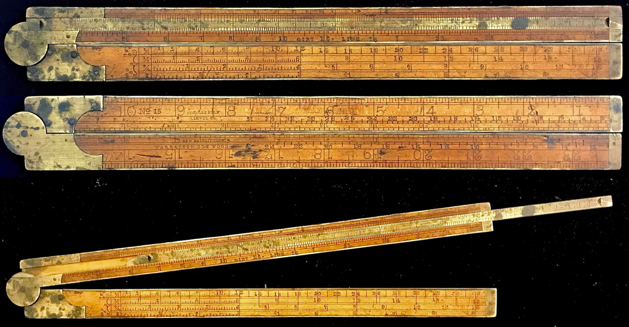
A carpenter’s slide rule has four scales which came to be labeled A, B, C, and D. The B and C scales are both located on the slide of the rule. The A scale is on the stock, above B. The fourth scale, D, is on the stock below C. The first three scales are each two-decade logarithmic scales that start at “1” on the left, and go to “100” on the right. However, the D scale is a single-decade logarithmic scale.
But what makes the carpenter’s rule stand out even further is the fact that the D scale starts at “4” on the left and ends at “40” on the right. Due to the fact that timber measurements involve boards and logs whose cross sections are usually measured in units of inches, and whose lengths are usually measured in feet, then there is always a factor of 12 floating around in the calculations. By having the “12” on the D scale near the center of the rule, this conversion factor could be dealt with much more efficiently in general timber calculations.
Below is an image of a carpenter’s rule from the 1800s. This is a Model No. 15 made by the Stanley Rule and Level Company of New Britain, Connecticut in the U.S., probably made within the first few years of its production.86 The Model 15 was first offered by Stanley in 1855.87 Aside from the Palmer’s Calculating Scale of the 1840s, the earliest slide rules made in the U.S. appear to have been carpenter’s rules of this type (not necessarily by Stanley).88
An example calculation on the carpenter’s rule, as might have been performed in the 1800s, would go something like this:
Determine the volume in cubic feet given by a timber that is 30 inches wide, 8 inches thick, and 12.7 feet long.
The solution begins by finding the “mean square” of the board. This is the length \(m\) of the side of a square that would create the same cross-sectional area as the board in question. So if the board has width \(w\) and thickness \(t\), then \(m^2 = w\times t\), or \(m = \sqrt{w\times t}.\) (The lengths \(w\), \(t\), and \(m\) are all in inches.) To find \(m\) on the carpenter’s rule, the user takes the width and lines up its value on D with the same value on C. Then, under the thickness on C we find the mean square on D. For our case we get a mean square of 15.5 inches.
To see how it works, start with \(m=\sqrt{wt}\). Now take the ratio \(w/m\) = \(w/\sqrt{wt}\), or \(w/m\) = \(\sqrt{w}/\sqrt{t}\). Re-arranging,
\[ \frac{\sqrt{w}}{w} = \frac{\sqrt{t}}{m}. \]
But since numbers on C go like the square of numbers on D, then lining up \(w\) on C above \(w\) on D is the same ratio as lining up \(t\) on C above \(m\) on D. So dialing in \(w\) and \(t\) as we did above, \(m\) can be read off directly.89
Now that the mean square of the board has been established, to complete the calculation on the carpenter’s rule, we take the length \(L\), which is in feet, on C and line this up with the 12 on D. Then, above the value of \(m\) on D will be the volume in cubic feet on C. For our numbers we get a volume of 21.2 cubic feet. In essence, we are finding the volume \(V\) in cubic feet using
\[ V =( m/ 12)^2 \times L \] where we remember that \(m\) is in inches and thus needs to be converted to feet. But, thinking in terms of ratios, this is equivalent to writing
\[ \frac{L}{12^2} = \frac{V}{m^2} ~~~~~~{\rm or}~~~~~~ \frac{\sqrt{L}}{12} = \frac{\sqrt{V}}{m} \]
such that by the identical argument we used earlier, \(m\) is found by the settings on the slide rule as just described.
This is simply one example of a typical calculation performed with the carpenter’s rule, and of course there are many others. Another common example is to compute the volume of a round log of diameter \(D\). The volume is \(V =\pi/4\times D^2 \times L\). Rather than deal with diameters and factors of \(\pi\), the logger would more easily measure the circumference of the log with a rope or string. Then, folding the rope in two, and folding a second time, gives a length of rope called the “quarter girth”, or often just called the “girt” of the log. This length could be measured directly using the inch scales on the (possibly unfolded) carpenter’s rule. The length of the log in feet would be set against the 12 on the D scale (which in this context is called the Girt Line), and then opposite the girt distance on D would be the volume of the log on C. But note that this is an approximation and will be off by a factor of \(4/\pi\). (The girt is one-fourth of the circumference, or \(\frac14 \pi D\); hence, \(V =4/\pi \times {\rm girt}^2\times L.\)) But, in the logging business, this overage of the calculated volume would be used to account for the excess wood that would be trimmed away when the tree was shaped and was often ignored for this reason, yielding a simpler calculation to be performed at the logging site. In the image of the Stanley rule above one can see the words “Girt Line” surrounding the 12 mark on the D scale.
The Stanley No. 15 also has other scales on it for the convenience of the carpenter, such as length scales in fractions of an inch, and lines of values used when making octagonal cuts (E and M lines), and so on. But these do not involve direct use of the slide rule capabilities of the rule, merely providing useful constants or gauge mark values.
8.22.2 An Engineer’s Rule
The late 1700s and early 1800s also saw the rapid development of the steam engine. The Scotsman James Watt improved upon the design and efficiency of the engine and his famous patent of 1769 – “A New Invented Method of Lessening the Consumption of Steam and Fuel in Fire Engines” – contributed substantially to the initialization of the Industrial Revolution. Watt was immortalized when the standard unit of “power” was named after him. (Think “100 Watt light bulb”, for instance.) He relocated to the Birmingham, England, region in 1774 soon after English manufacturer and engineer Matthew Boulton, the manufacturer of the Soho Works in Birmingham, took over a share in Watt’s patent.90 After the patent was extended by an act of Parliament, Watt and Boulton worked together for over 25 years to make rapid progress with the steam engine. Soho – an abbreviation of “South House”, denoting that it was located to the south of Handsworth, just outside of Birmingham – became famous for their work, and the slide rules that they developed for their activities became known as “Soho rules”.
The typical scale layout of the Soho rules – also known as “engineer’s rules” – were very similar to those of the earlier carpenter’s rules with the exception of the D scale. While the carpenter’s rule has a D scale that runs from 4 to 40, the engineer’s rule has a D scale that runs from 1 to 10.
A standard Soho rule is of a very “normal” design with a slide attached to a stock and four standard scales A, B, C, and D. Other rules with the same set of scales, like the Routledge Engineer’s rule shown below, are similar to our earlier example of a carpenter’s rule, with a slide attached to one leg of a folded measurement scale.
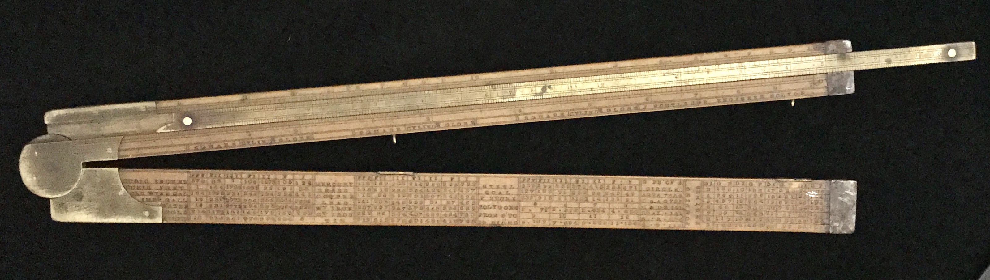
On one side of the folded rule is a two-foot scale. If the brass slide is fully extended, the total length of the ruler is three feet, or one yard. The other side of the rule is the computational side, where the B/C scales are on the brass slide, with the A above and the D scale below the slide. With D running from 1 to 10, squares and square roots of any number readily can be found for numbers on A, and also can be used in calculations using the slide. This made the slide rule more practical for use in many general calculations.
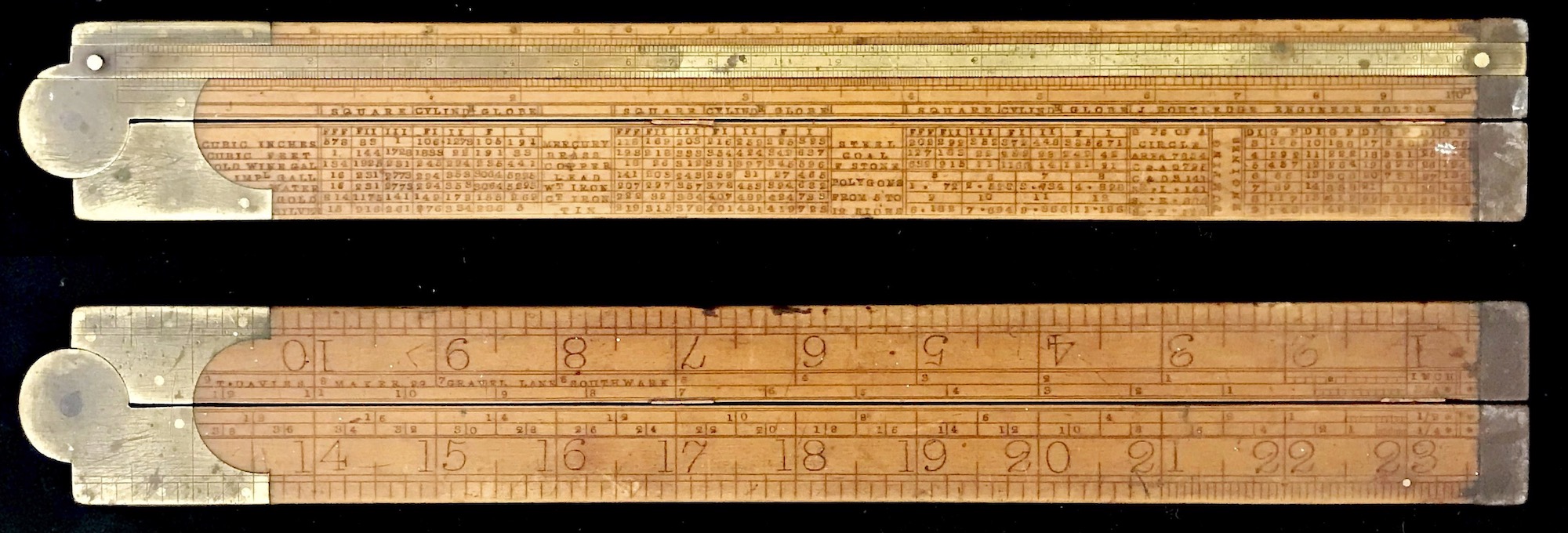
Like the carpenter’s rule, the engineer’s rule became a common instrument for steam engineers and other general tradesmen of the day and could be found in use into the early 20th century. Also like our carpenter’s rule which had special scales useful in the timber industry, the engineer’s rules typically have a table of useful constants and gauge marks helpful in the engineering trades of the day.
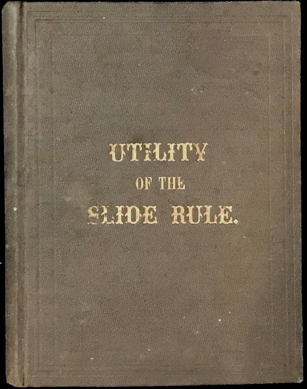
Both of these styles of early slide rules were in full use in the 1800s. A nice little book entitled The Utility of the Slide Rule, by Arnold Jillson, written in 1859, describes various calculations that can be done with both styles of slide rule. Part I of the book is devoted to the use of the carpenter’s rule, while Part II is for the engineer’s rule. Pages from a copy of the 1874 edition are shown below. In particular, note how Jillson talks about the two types of rules in his Preface.
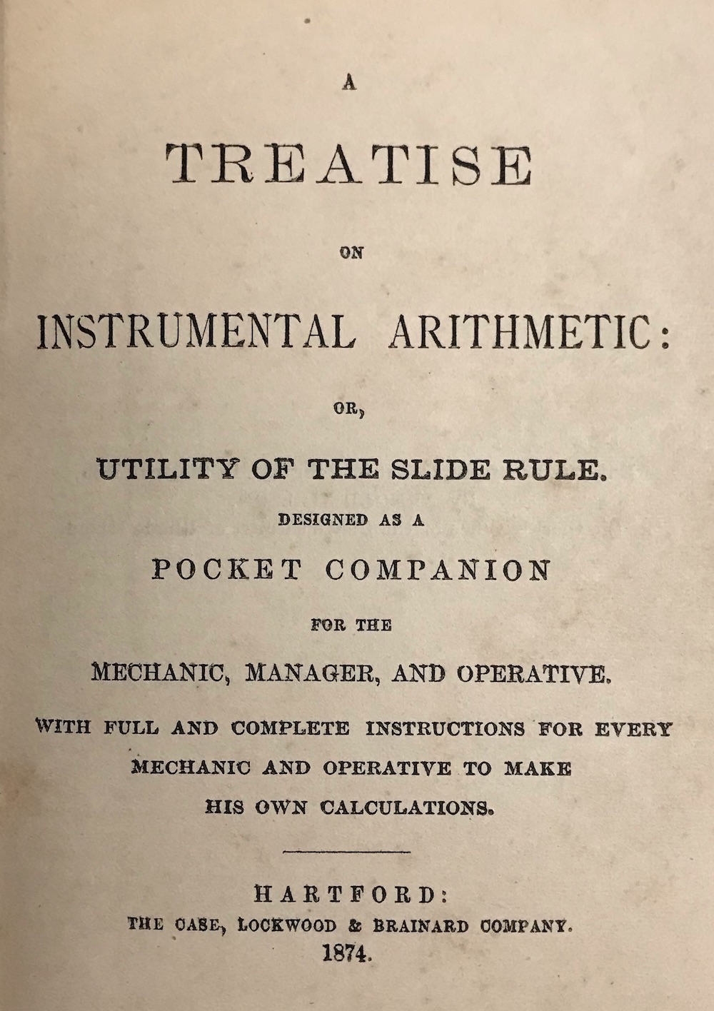
/
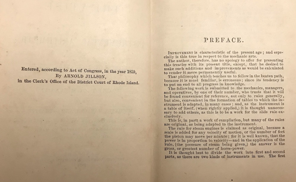
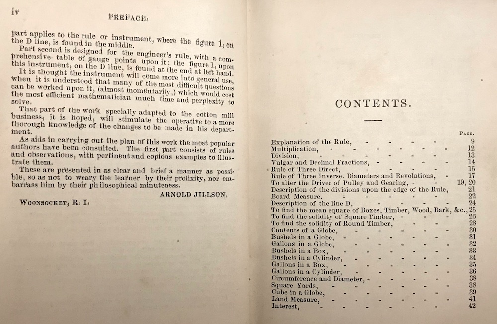
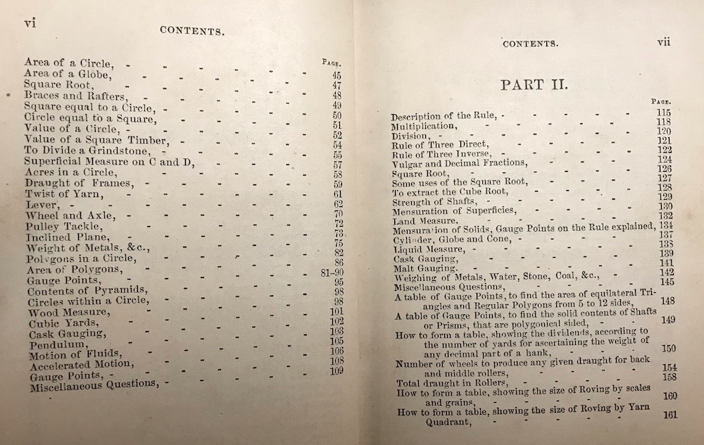
The Utility of the Slide Rule, by Arnold Jillson. Top to bottom, left-to-right: Cover, Title Page; Preface, Contents Part I, Part II; Sample Text
Florian Cajori, A History of the Logarithmic Slide Rule, The Engineering News Publishing Company, New York (1909) p28.↩︎
Within a few years of production, Stanley added “U.S.A.” in the address given on the rule. Our rule does not have “U.S.A.” in the address.↩︎
Philip E. Stanley, Boxwood and Ivory: Stanley Traditional Rules, 1855-1975, Stanley Publishing Co., Westborough (1984).↩︎
Thomas Wyman, “When Was The First Slide Rule Produced In The United States?”, Jour. Oughtred Soc., 23.1, p38 (2014).↩︎
One need not have a carpenter’s rule to perform this calculation – it works using a standard slide rule substituting the modern B and D scales in place of the carpenter’s rule’s C and D scales.↩︎
Kingsford, P. W.. “James Watt.” Encyclopedia Britannica, June 9, 2023. https://www.britannica.com/biography/James-Watt.↩︎
Now, slide the cursor over to 3.4 on the D scale; you should see 3.4 on the B scale under the cursor. We have arrived at the same setting of the slide as when we used ratios, as should be expected.↩︎
Mannheim actually added a cursor to his slide rule in 1851, a year after presenting his new scale arrangement.↩︎
8.22.3 Comments on Scale Development
Let’s summarize what we’ve learned about the development of these early slide rules. Start with the Gunter scale, which immediately followed the invention of the logarithm and its early development by John Napier and Henry Briggs. This was at first a curiosity to most people, but the Gunter scale was immediately seen useful in navigation, for example, especially when logarithmic scales of trigonometric functions were added into the mix. This, after all, was an impetus for the development of logarithms by Napier. As the slide rule instrument slowly became known throughout England and Scotland in the 1600s and 1700s, industries came to use variations of such scales in their work, such as in cask gauging, excise taxation, and the timber industry. These industries had unique arrangements of Gunter scales – especially the first two just mentioned – including what we would now call folded scales and the occasional reversed scale. In fact, later Excise Officer’s gauging rules even had 1/2-decade scales which on future slide rules (the early Picketts, Post’s Versalog, and the Faber Castell 2/83N come to mind) might be called R1/R2, or W1/W2, for example. Many early slide rule makers labeled their scales with A, B, C, and so on, though there did not yet appear to be any strong convention used among the makers.
In 1677 Henry Coggeshall “standardized” a slide rule scale set into what is now called the “carpenter’s rule”, with four logarithmic scales also labeled A, B, C, and D. He made the factor of 12 a central point on the D scale, convenient for the conversion of inches to feet, while the A and B scales could also be used for more general calculations. The D scale ran from 4 to 40 (one decade) left-to-right, while A, B, and C ran from 1 to 100 (two decades) left-to-right.
It is interesting to me that in the books of the late-1700s and 1800s that I have access to, the calculations are almost always developed in terms of “ratios”. That is, instead of directly computing a quantity such as the “mean square” – \(m=\sqrt{a\cdot b}\) – as I was taught to do in school, a ratio would be developed where the answer could be found using the law of ratios on the slide rule. For example suppose \(a\) = 3.4 and \(b\) = 23.2 in our equation above. Compare the two techniques, here using a standard modern slide rule:
Using Ratios – Re-write the equation \(m=\sqrt{ab}\) (or \(m^2 = ab)\) as \(a/a^2 = b/m^2\). Now, note that the numbers on the A scale vary like the square of the numbers on the D scale. Hence, by lining up 3.4 on the A scale with 3.4 on the D scale, then by finding 23.2 on the A scale we see below it 8.88 on the D scale – the law of ratios.
Compute Directly – Start with the slide reset (indices aligned on A and B, say). Move the cursor to the first number, 3.4, on A. Align the index on B to the cursor. Move the cursor to the second number, 23.2, on B. On A will be 3.4 times 23.2. Below, on D, will be the square root of this answer: 8.88.91
The carpenter that was taught how to do the first version above likely would not have been taught – or likely would not have even been aware of – how to re-write an equation and use these steps to arrive at the answer. He was simply shown how to do this particular calculation on the slide rule and (perhaps) marveled at the fact that it worked. What I find in the early instruction books is that no mention is made as to why the methods for using the slide rule this way actually work. The books tend to only give precise instructions, along with ample examples for people to practice, on how to perform a particular calculation (such as volume of a cylinder, conversion of gallons to bushels, etc.). But from reading these directions, it seems evident that the use of the slide rule scales for finding ratios of quantities was perhaps the most common practice by those who understood the mathematics.
Since the carpenter’s rule had the folded D scale with 12 in the middle, then its usefulness in other applications wasn’t necessarily obvious to others outside the timber industry. But this changed with the engineer’s rule. Here, the D scale started with 1 and ran to 10, while the A, B, and C scales remained as two-decade scales from 1 to 100. Even though any general calculation could be arrived at with the carpenter’s rule as well, the direct 1-to-1 correspondence of the scales on the engineer’s scale likely made general calculations much more intuitive, more along the lines of our second example above. This must have been instrumental in the eventual move toward more direct techniques of general computation using a slide rule.
The last step in the transformation of the early rules to the modern slide rule was performed by Amédée Mannheim. The carpenter’s and engineer’s rule each has a slide with a B scale and a C scale. But upon close inspection one notices that these two scales are actually just one scale, repeated at the top and bottom of the slide. The reason for this was that when one lines up a number on A with a number on B, the eye can easily set the two scales fairly accurately due to the proximity of the two scales. To read off a number on D with a number on the slide, a separate set of lines were drawn on the bottom edge of the slide called the C scale. This way the eye can compare and interpolate results between hatch marks on these two scales as well. But in reality, B and C are simply the same scale.
I believe that Mannheim, on the other hand, must have realized two things. Firstly, it was inefficient to repeat the B scale with a C scale, both on the slide, where a different scale could be added instead. If the C scale were a single-decade scale like the D scale, then C and D could be used for general calculations often with higher accuracy than using the A and B scales, and also many computations requiring squares or roots of numbers could be performed more readily as well. But secondly, he realized that if a “cursor” were added to the slide rule, then the same interpolation of results by eye could be accomplished not only between the B and D scale, say, but also between any of the four scales.92 So, with Mannheim’s new set of scales and – perhaps even more importantly – his addition of a cursor, the transformation to the Modern slide rule was essentially complete. Future general purpose slide rules would have new scales created and added to enhance the Mannheim design, making them ever more powerful yet familiar to the user.
Modern General Purpose Slide Rule Scale Development. – labels within
[and]denote scales on the slide.The labels A, B, C, and D below refer to the modern labels, not necessarily labels used at the time. DF4 is a 1-decade scale “folded” at 4.
The carpenter’s rule was an inspiration for the engineer’s rule, which itself became a precursor to the more modern slide rule layout instigated by Mannheim. The seemingly slight improvement of the scale arrangement by Mannheim in 1850, along with his use of a built-in cursor in 1851 for accurate alignment of the scales, brought about a very robust instrument useful not only to the French military in Mannheim’s case, but also to a variety of future engineers, scientists, bankers, builders, industrialists, farmers and agriculturalists, and more.
For some nice overviews of the carpenter’s and engineer’s rules and their variations, and a bibliography of early instruction books, see