8.18 Thacher’s Calculating Instrument
Need that extra digit in the answer and having trouble interpolating between those marks on your 10-inch slide rule? Thacher’s Calculating Instrument may just be the solution for you.
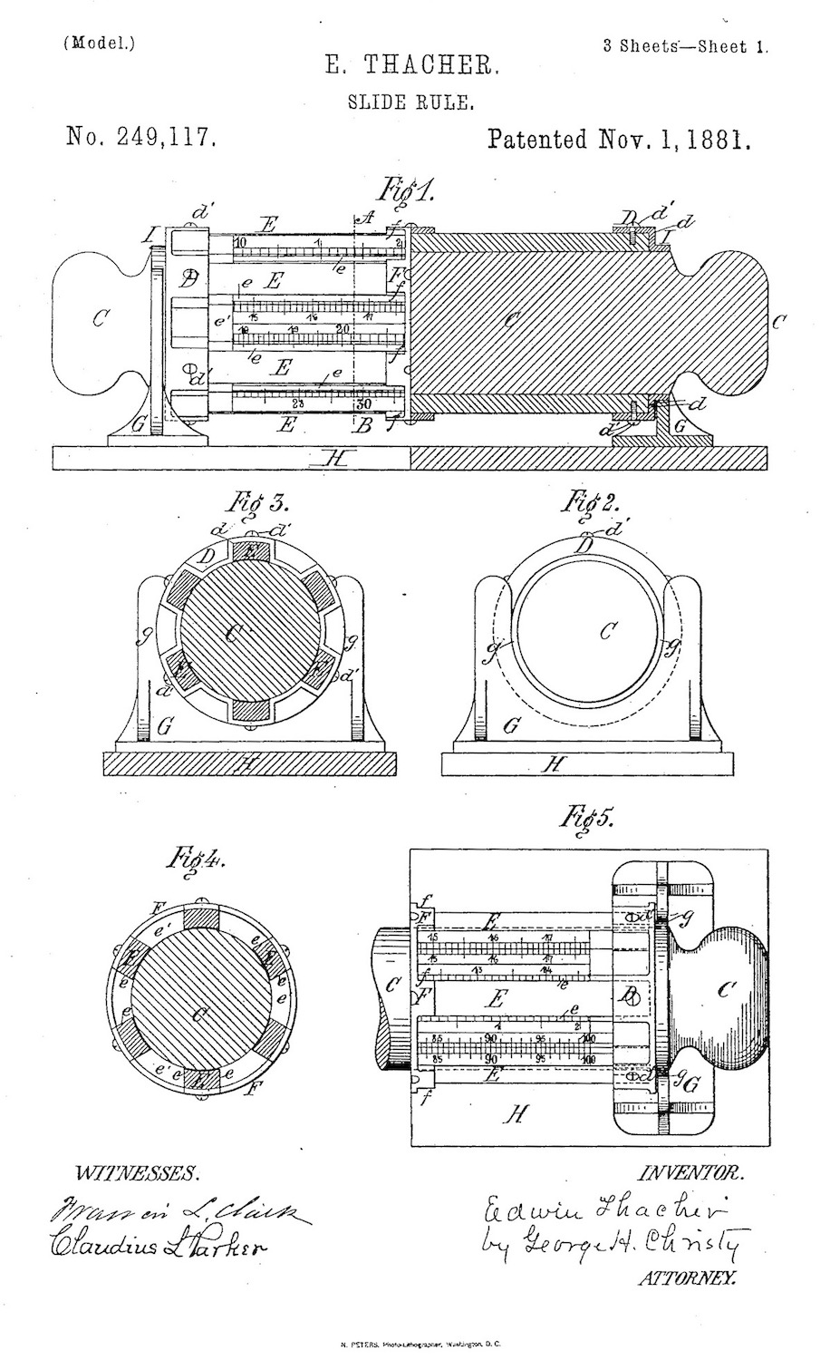
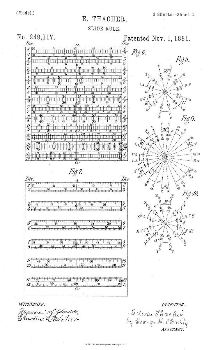
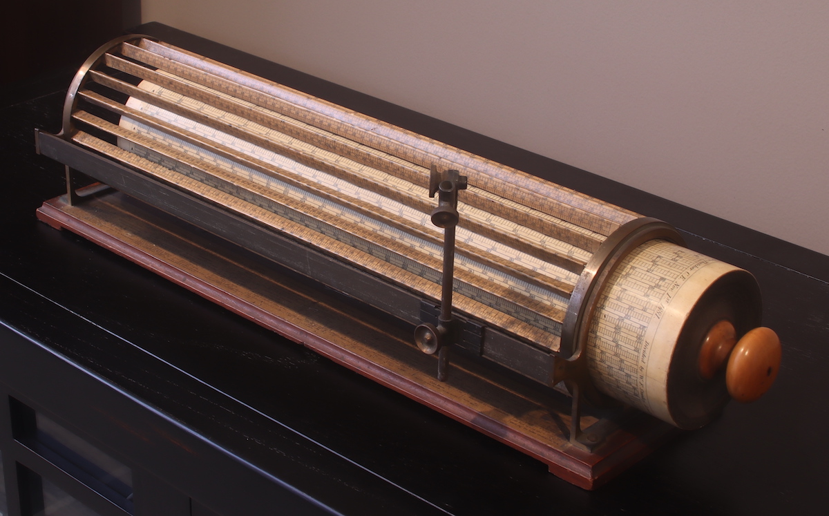
Patented in 1881 by Edwin Thacher of Pittsburgh, Pennsylvania, the ominous looking device has the equivalent length of a 30-foot slide rule and can compute multiplication and division problems that can be read off with 4-to-5-digit accuracy. Two years earlier, a somewhat similar looking device – the Fuller calculator, or, Fuller’s Spiral Slide Rule – was patented by George Fuller of England. But these are two very different approaches to the same problem. The Fuller, which is described in Helical Slide Rules, is comprised of two helical logarithmic scales on two concentric cylinders that are slid back and forth to perform calculations. Thacher’s idea was to make a set of very long linear logarithmic scales that are divided up into segments, but placed along the surfaces of two concentric cylinders that can be rotated and slid longitudinally to perform the same function. The device can sit on a table and is easily manipulated in place, while the Fuller design required that device be hand held. (Later Fuller model refinements included a rod that could be inserted into its handle to support the slide rule at an angle for easier use.) For many years the Thacher and the Fuller were used for precision calculations required by engineers, bankers, tax assessors, and others. By 1891 Keuffel and Esser had purchased the rights to Thacher’s patent and started to produce and sell the slide rule as one of their very first American-made models.
The Thacher line consisted of three different models. The first model, designated Model 1740/1741, was produced between 1891 and 1899. The model numbers of K&E were changed in 1900, and the Thacher became Model 4012/4013 and included a slightly redesigned frame. The 1740 and 4012 were the standard item, while models 1741 and 4013 came with an attached sliding magnifier for easier reading of the scales. The Thacher in the collection, shown above, was acquired with the help of the International Slide Rule Museum (ISRM). It is a Model 4013 and has K&E Serial Number 2179, indicating that it was most likely made in very early 1907. Models 4012/4013 saw minor changes in 1927, and were branded N4012/N4013. N4013 was absent from the K&E catalogue beginning in 1942, while N4012 continued until 1952.
8.18.1 Edwin Thacher
Born in DeKalb, New York, in 1839, Edwin Thacher was graduated with high honors from the Rensselaer Polytechnic Institute in Troy, NY, in 1863.54 Following service through the Civil War, during which he became assistant engineer of the United States military railroads, Thacher worked in connection with the construction of the Cincinnati branch of the Louisville, Cincinnati & Lexington Railroad. By 1868 he had become assistant engineer of the Louisville Bridge Company, which was then building a bridge across the Ohio River from Louisville into Indiana. Soon called the “Fourteenth Street Bridge” by locals, this was the longest iron bridge in the United States at that time, with 27 spans covering a total length of one mile.55 In 1870, once the bridge was open and operational, Thacher became a computing engineer of the Louisville Bridge & Iron Company. The rest of his career was devoted mostly to structural calculations associated with bridge construction. In 1881 he patented his slide rule design in his quest for fast and reliable engineering calculations.56 By 1883 he was hired as Chief Engineer for steel tycoon Andrew Carnegie’s famous Keystone Bridge Company, of Pittsburgh, PA.
As early as 1889 Thacher became interested in concrete-steel construction. In 1894, as a partner in the firm of Keepers & Thacher, his firm designed the concrete-steel arch over the Kansas River at Topeka, which was a very notable design in its day. It was during this time that he also became known for his “Thacher bar” used in reinforced concrete construction, which became a standard reinforcment technique in the new industry.
After other projects in Alabama and Detroit, Edwin moved to New York City in 1900 to form the Concrete Steel Engineering Company with William Mueser, another bridge engineer who had immigrated to the U.S. in 1893, and who had designed the first reinforced concrete arch bridges in New York, New Jersey, Pennsylvania, and the District of Columbia.57 Thacher worked with Mueser until retiring in 1912, spurred by his failing eye sight. Edwin Thacher died in 1927 at his home in New York City.
 |
 |
 |
8.18.2 The Thacher Layout
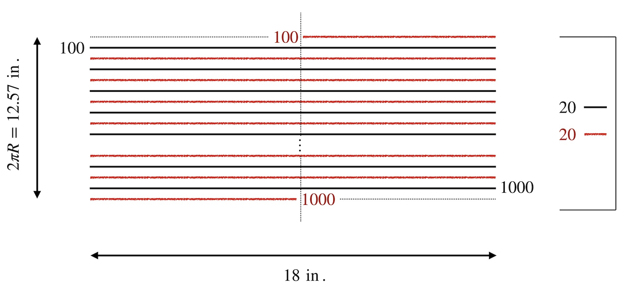
The basic scale on the Thacher Calculating Instrument is a 360-inch logarithmic scale that is divided into 20 18-inch segments. The diameter of the cylinder is 4 inches and hence has a 12.57 inch circumference. The values on the scale are labeled to avoid decimal points, with numbers running from 100 to 1000. Let’s determine where the “break points” are for this major scale, called the “A” scale on the Thacher. Suppose xL and xR represent the left and right end points of each segment, in inches, and xM is the midpoint between them. The following code generates a table that gives the values on the logarithmic scale at the beginning (AL), middle (AM), and end (AR) of each of the 20 segments.
L0 = 360
nBar = 20
Segment = c(1:nBar)
offset = 0
xR = L0/nBar*Segment+offset
xL = xR-L0/nBar
xM = (xL+xR)/2
AL = 10^((xL)/360)*100
AM = 10^((xM)/360)*100
AR = 10^((xR)/360)*100
AL = ifelse(AL< 100,AL*10,AL)
AR = ifelse(AR>1000,AR/10,AR)
kable(round(cbind(Segment,xL,AL,xM,AM,xR,AR),1),format = "pandoc")| Segment | xL | AL | xM | AM | xR | AR |
|---|---|---|---|---|---|---|
| 1 | 0 | 100.0 | 9 | 105.9 | 18 | 112.2 |
| 2 | 18 | 112.2 | 27 | 118.9 | 36 | 125.9 |
| 3 | 36 | 125.9 | 45 | 133.4 | 54 | 141.3 |
| 4 | 54 | 141.3 | 63 | 149.6 | 72 | 158.5 |
| 5 | 72 | 158.5 | 81 | 167.9 | 90 | 177.8 |
| 6 | 90 | 177.8 | 99 | 188.4 | 108 | 199.5 |
| 7 | 108 | 199.5 | 117 | 211.3 | 126 | 223.9 |
| 8 | 126 | 223.9 | 135 | 237.1 | 144 | 251.2 |
| 9 | 144 | 251.2 | 153 | 266.1 | 162 | 281.8 |
| 10 | 162 | 281.8 | 171 | 298.5 | 180 | 316.2 |
| 11 | 180 | 316.2 | 189 | 335.0 | 198 | 354.8 |
| 12 | 198 | 354.8 | 207 | 375.8 | 216 | 398.1 |
| 13 | 216 | 398.1 | 225 | 421.7 | 234 | 446.7 |
| 14 | 234 | 446.7 | 243 | 473.2 | 252 | 501.2 |
| 15 | 252 | 501.2 | 261 | 530.9 | 270 | 562.3 |
| 16 | 270 | 562.3 | 279 | 595.7 | 288 | 631.0 |
| 17 | 288 | 631.0 | 297 | 668.3 | 306 | 707.9 |
| 18 | 306 | 707.9 | 315 | 749.9 | 324 | 794.3 |
| 19 | 324 | 794.3 | 333 | 841.4 | 342 | 891.3 |
| 20 | 342 | 891.3 | 351 | 944.1 | 360 | 1000.0 |
A second version of the same scale is also found on the inner cylinder. It is made of an additional 20 segments, but this scale begins in the middle of its first segment. Such a layout is generated by roughly the same code, but setting the parameter offset = L0/nBar/2. Here is the result58:
| Segment | xL | AL | xM | AM | xR | AR |
|---|---|---|---|---|---|---|
| 1 | -9 | 944.1 | 0 | 100.0 | 9 | 105.9 |
| 2 | 9 | 105.9 | 18 | 112.2 | 27 | 118.9 |
| 3 | 27 | 118.9 | 36 | 125.9 | 45 | 133.4 |
| 4 | 45 | 133.4 | 54 | 141.3 | 63 | 149.6 |
| 5 | 63 | 149.6 | 72 | 158.5 | 81 | 167.9 |
| 6 | 81 | 167.9 | 90 | 177.8 | 99 | 188.4 |
| 7 | 99 | 188.4 | 108 | 199.5 | 117 | 211.3 |
| 8 | 117 | 211.3 | 126 | 223.9 | 135 | 237.1 |
| 9 | 135 | 237.1 | 144 | 251.2 | 153 | 266.1 |
| 10 | 153 | 266.1 | 162 | 281.8 | 171 | 298.5 |
| 11 | 171 | 298.5 | 180 | 316.2 | 189 | 335.0 |
| 12 | 189 | 335.0 | 198 | 354.8 | 207 | 375.8 |
| 13 | 207 | 375.8 | 216 | 398.1 | 225 | 421.7 |
| 14 | 225 | 421.7 | 234 | 446.7 | 243 | 473.2 |
| 15 | 243 | 473.2 | 252 | 501.2 | 261 | 530.9 |
| 16 | 261 | 530.9 | 270 | 562.3 | 279 | 595.7 |
| 17 | 279 | 595.7 | 288 | 631.0 | 297 | 668.3 |
| 18 | 297 | 668.3 | 306 | 707.9 | 315 | 749.9 |
| 19 | 315 | 749.9 | 324 | 794.3 | 333 | 841.4 |
| 20 | 333 | 841.4 | 342 | 891.3 | 351 | 944.1 |
| 21 | 351 | 944.1 | 360 | 1000.0 | 369 | 105.9 |
On the main cylinder of the Thacher, these two scales are engraved in an interleaved fashion. The sketch below depicts the unwrapped surface of the cylinder with the two scales, one which begins in the middle of the cylinder (in red) and the other which begins at the left end of the next line (in black). The two systems “leap frog” each other until their ends meet up after one revolution of the cylinder.
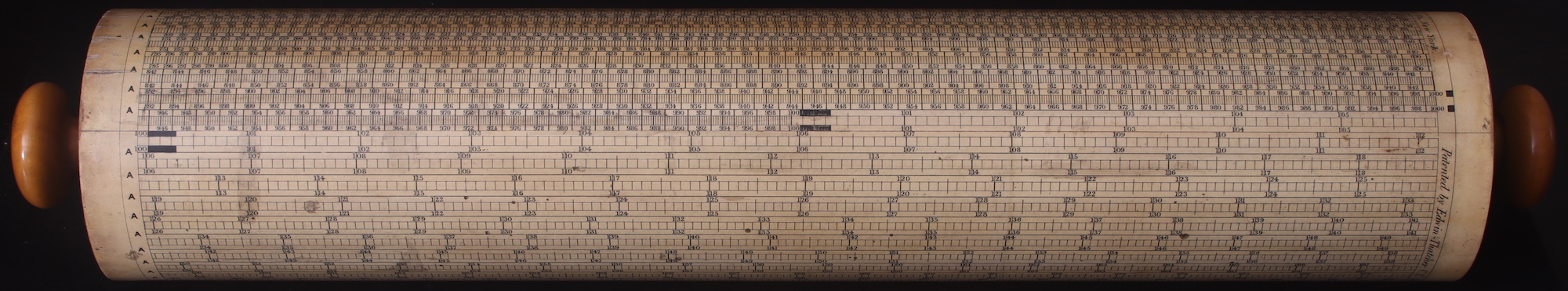
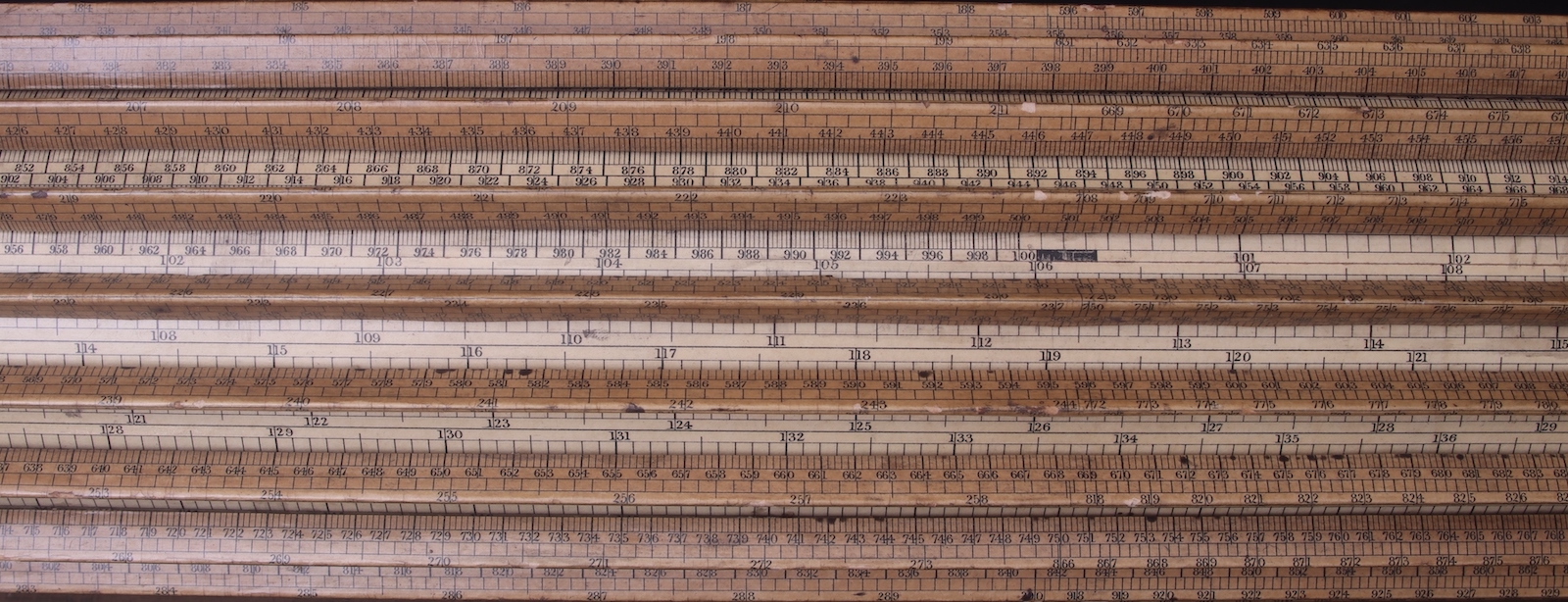
Below is an image of the inner cylinder which has been removed from the instrument. The scale indices (100/1000, on both the first and second scale set) are marked by dark black bars so that they are easily found by the user.
This main cylinder is free to rotate and move along its axis while being supported by a system of 20 bars that span parallel to the axis of the cylinder. An image of the system of bars, sometimes referred to as “the envelope”, is shown in the image below.
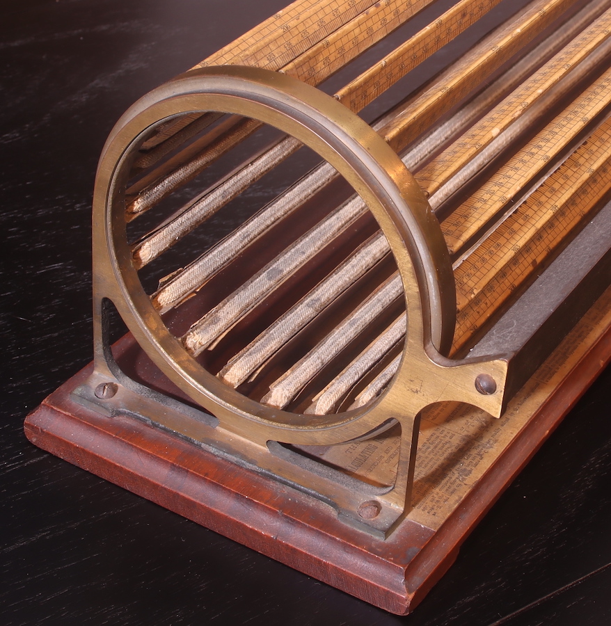
These bars, too, are connected at their ends to slip rings which allow the entire support structure to rotate about its axis as well. Thus, the user can grab the rings on the outer edges and rotate the entire envelope of bars to find a particular value on the bars to view. Then, by grabbing the knobs of the inner cylinder, it can be separately rotated and slid back and forth in order to line up a number on the cylinder with a number on the bars.
The so-called “bars” are triangular in shape and the bottom edges of each bar, which are coated with soft material, come into contact with the inner cylinder, allowing the inner cylinder to gently slide and rotate within the envelope. Thus, the inner cylinder can be viewed through “windows” between the bars, as depicted in the image below.

On the slanted faces of each bar are additional logarithmic scales. The set of scales on the inner cylinder are labeled “A” on the Thacher. On each of the faces of the bars, the scales are referred to as “B” (closer to A) and “C” (further from A). The B scales are just replicates of the A scales, one on the “upper” bar faces where the index starts in the middle, and the other on the “lower” bar faces where the index starts on the left end. If one lines up the middle index (100) on A with the same middle index on the upper B scale, and rotate the inner cylinder slightly so as to simultaneously reveal the index on the left-hand index on A, it will be opposite the left-hand index on the lower B scale; and then A and B scales are found to be totally opposite each other everywhere on the instrument.
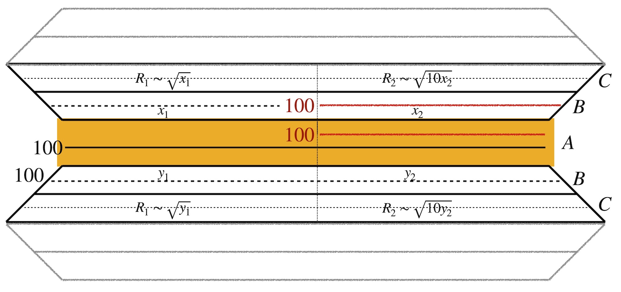
The C scales are for finding square roots of numbers, but this will take a little further discussion. The best way to think of this is to imagine not a square scale, such as the standard A/B scales on a Mannheim slide rule, but rather a set of square root scales, as might be found on a Post Versalog or other advanced slide rules, sometimes called the R1 and R2 scales, or perhaps W1/W2 as on some European models. Since a portion of the C scale is found on each side of each bar, it can be thought of as two distinct scales, one that runs from \(\sqrt{10}\) to \(\sqrt{100}\) and one that runs from \(\sqrt{100}\) to \(\sqrt{1000}\). Suppose we find a number on the B scale above the window. Then, if that number is to the left of the cylinder’s middle, the number above it on the C scale will be the actual square root of the number on B. If, though, the number on B is to the right of the cylinder’s middle, the number above it on C will be the square root of 10 times the number on B. The scales below the window act exactly the same way.
8.18.3 Performing a Calculation
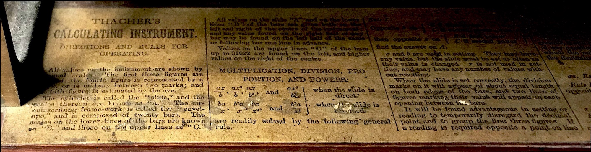
The fact that there are two slightly offset 30-foot scales on the inner cylinder might give the user the impression that using this slide rule is going to be a complex operation. So, just in case one forgets how to use the instrument, instructions can be found on its base.
However, by now, the user – well versed in the logarithm and standard slide rule operations – might already be able to see how to use the slide rule: From the position of having all indices aligned, move an A index to a number on B, find a second number on A and opposite on B will be the product of the two. And there you have it! And note that with two sets of scales on A and on B, then when one A scale is slid by a certain amount (indicating a multiplication, say) then the other interleaved A scale is automatically slid by the same amount. The result one is looking for can be found on either of these A scales. However, if the answer being sought on one A scale is “off scale” because the slide is extended, then the other A scale should be “on scale” and the answer visible. Thus, one should be able to find a result without having to “reset the slide” as is commonly necessary in most linear slide rule calculations. This would be the purpose of having two identical, but shifted, logarithmic scales on the slide and on the bars. They operate in a somewhat similar way to a folded scale (CF/DF) on a more modern linear slide rule.
And as for the C scale, since this is equal to the square root of values found on the B scale, then basic calculations involving squares and square roots also can be performed.
As an example we show a close up below of the Thacher in which we have aligned two numbers: the middle index on A is aligned with “500” on the upper B scale. You can find these two numbers by looking just to the left of the long dark bar, found to the right of center of the photo. Now suppose we wanted to calculate 97.08 % of 500. With the present setting, just look for 9708 on B, which is on the same line and to the left, and under this number we find the answer on B: 4854, or rather 485.4. Clearly many other products with 500 can easily be found with a glance at this figure.
As another example, suppose that we need to calculate \(2.236^2\times 13.09.\) We estimate that the answer should be a a bit more than 4 times 13, or about 60. So, we find 2236 on the C scale as its square will be on the B scale – it is directly above the number 500! So, with the slide’s index already set to the square of 2.236, we look for 1309 on the A scale, which is located just a couple of windows below the index, and to the left. We find opposite 1309 on A, 6545 on B; or, 65.45. Check by computer: \(2.236^2\times 13.09\) = 65.446.
We can see how essentially any two 4-digit numbers can be easily multiplied and divided on the rule and a precise 4-digit answer can be achieved. (Perhaps even a 5-digit answer, with practice interpolating between the lines.)
Original instructions for the Thacher’s Calculating Instrument from 1884, which includes many examples, can be found online here:
and the ISRM has interesting Thacher information, including scales for making your own Thacher-style instrument, that can be found at the ISRM web site.
Other Thacher references:
- Bob Otnes, “Thacher Notes”, Jour. Oughtred Soc. 2.1 p21 (1993).
- Wayne Feely and Conrad Schure, “Thacher Slide Rule Production”, Jour. Oughtred Soc. 3.2 p38 (1994).
- Wayne Feely, “Update of Known Fuller and Thacher Rules”, Jour. Oughtred Soc. 5.1 p25 (1996).
8.18.4 Summary
The Thacher Calculating Instrument was a major achievement in the development of precision computational machinery that was readily available to industrial and financial institutions. The Thacher, and the Fuller as well, were two impressive instruments that were sold well into the 1950s and 60s and found in offices until the end of the slide rule era in the 1970s. It also makes a very fine looking antique on the desk at home.
From Wayne Feely, Jour. Oughtred Soc. 5.1 p25 (1996).↩︎
This section is adopted from information on the prabook and RPI web sites.↩︎
Kleber, John E., Encyclopedia of Louisville, University Press of Kentucky, p. 315 (2000).↩︎
Copies of the patent can be found online, such as at Google Books.↩︎
“Contextual Study of New York State’s Pre-1961 Bridges”, Mead & Hunt, prepared for New York State Department of Transportation, 1999.↩︎
Note that Segment 21 is actually the same line as Segment 1 on the cylinder.↩︎