1.2 Logarithms and Log Scales

Consider an arbitrary positive real number \(x\). As we just discussed, we can express \(x\) in terms of a base number – say, \(b\) – raised to a power \(p\):

\[ x = b^p. \] In standard mathematical language we say that the logarithm of the number \(x\) is the exponent \(p\): \[ \log_b x = p. \] The above expression is read, “The log, base \(b\), of \(x\) is equal to \(p\).” This definition leads to the following identity:

\[ x = b^{\log_b x}. \]

In mathematical terms we say that the function \(\log_b x\) is the inverse of the function \(b^x\) – if we start with \(x\) and find \(b^x\), and then take the logarithm using base \(b\) of the resulting number, we get \(x\) back again: \[ \log_b b^x = x. \]

In our earlier example we used \(2\) as a base, but the most common base to use, which is what typical slide rules have been based upon (no pun intended), is \(b\) = 10, or “Base 10”: \(x = 10^p\). The standard is simply to define the logarithm – or, the common logarithm – as that using Base 10:

\[ {\rm if} ~~ x = 10^p ~~~~ \longrightarrow ~~~~ \log x ~ \equiv ~ \log_{10} x = p. \]

In other words, ask, “To what power must you raise the number 10 in order to obtain the number \(x\)?” The answer, \(p,\) is the logarithm of \(x\) (simply called “log of \(x\)”). The convention is to write \(``\log x"\) when the base being used is 10. If it were another base, say \(2\), then the expression would be written \(\log_2 x\).

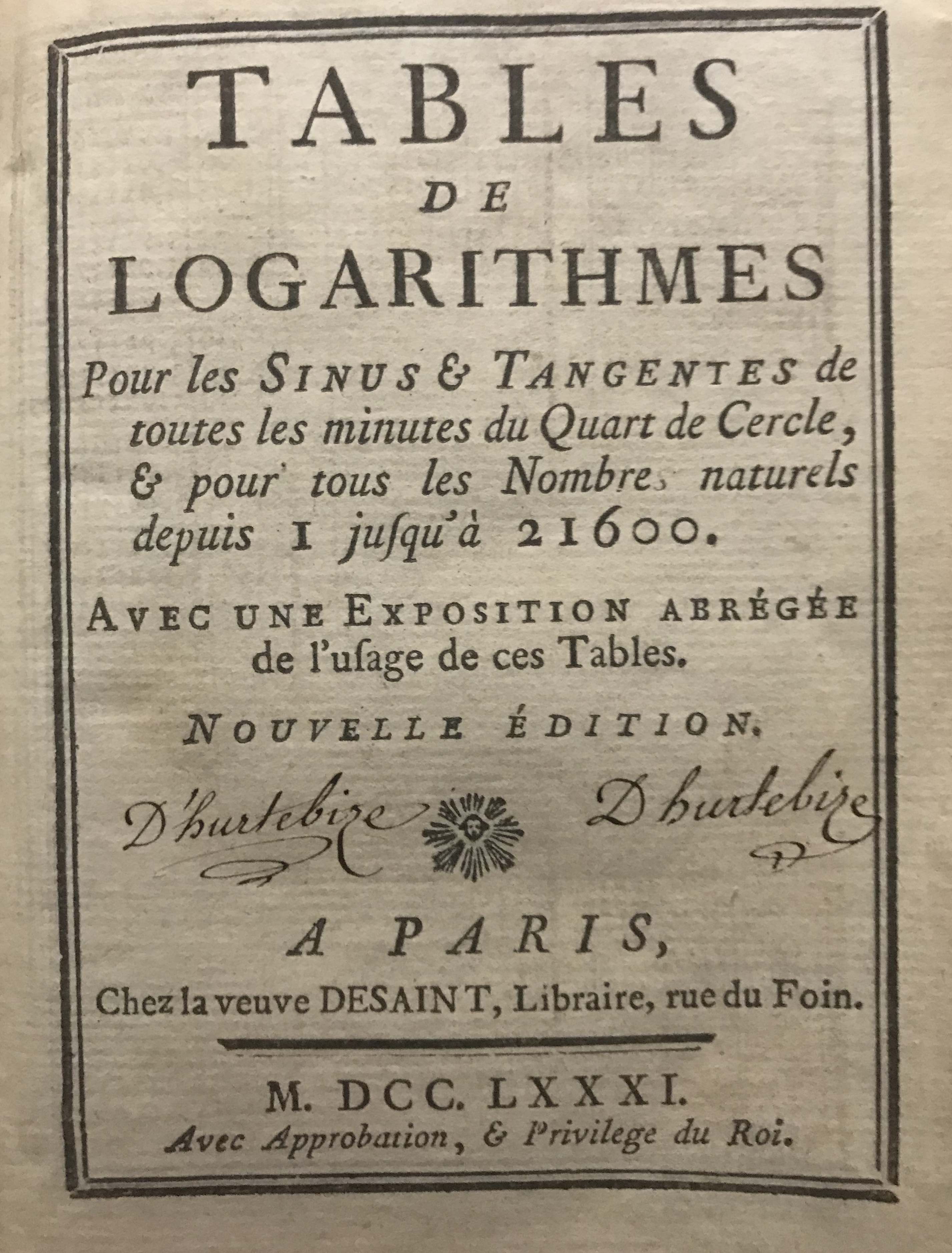
We saw earlier that any number raised to the power of “zero” is by definition “one”. Hence, log 1 = 0. That is, 1 = \(10^0\). The logarithm of a number greater than 1 will be a positive number. For example, \(10 = 10^1\) and \(100 = 10^2\), so \(\log 10 = 1\) and \(\log 100 = 2\). The logarithm of a number less than 1 will be negative: \(0.1 = 10^{-1}\) and \(0.01 = 10^{-2}\), hence \(\log 0.1 = -1\) and \(\log 0.01 = -2\). What about other, more general numbers? As we did before for our “Base 2” example, we can take the square root of 10, which is \(10^{1/2}\) = \(10^{0.5}\) = \(\sqrt{10}\) = 3.1623, and hence we can infer that \(\log 3.1623 = 0.5\). It can also be verified that \(10^{0.30103}\) yields 2.0000. Thus, \(\log 2\) is approximately equal to 0.30103. Precise values of the common logarithms of numbers can be calculated by using calculus, finite difference techniques, or other methods, and their values have been computed and tabulated with various degrees of accuracy over the past centuries. One such method for computing logarithms is presented in the next chapter. Books containing tables of values of logarithms were painstakingly produced and published for use in the types of calculations that will be described below; these books are also collectible and can be found in many used book stores.

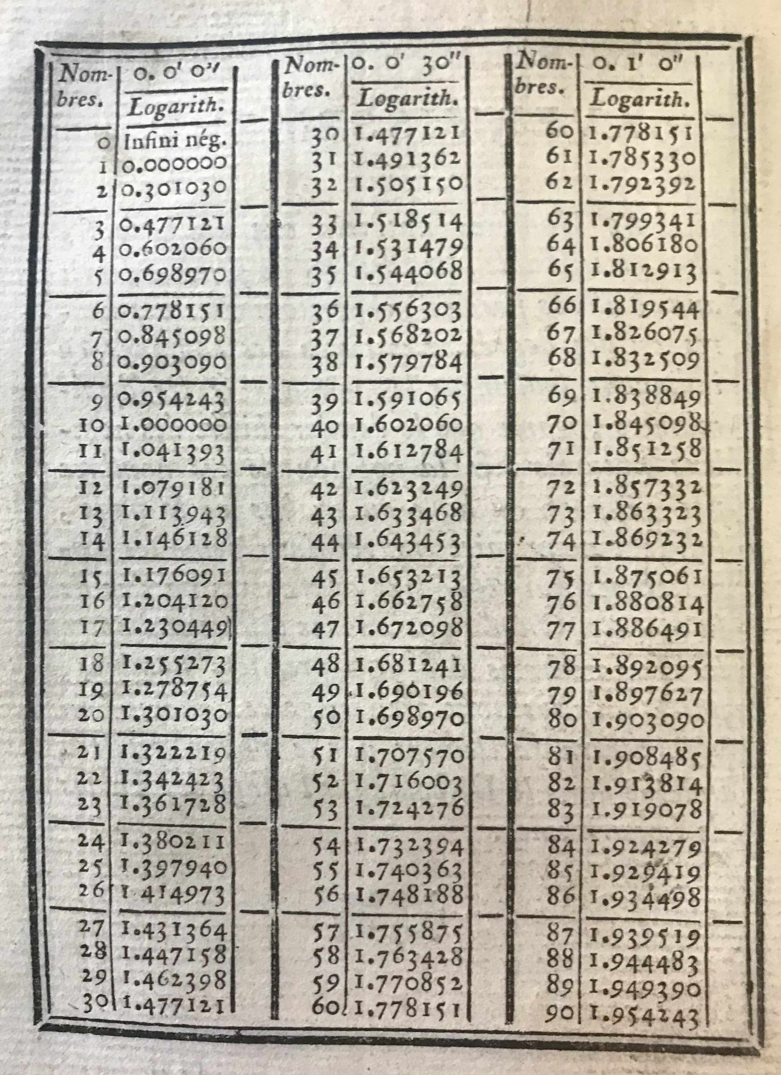A table of logarithms from the year 1781.3

Modern electronic computer languages have built-in algorithms that can produce logarithms of numbers to high accuracy. The following is a table of the Base 10 common logarithms of integer numbers between 1 and 100, similar to what can be found in a book of logarithms, but here generated by a modern personal computer:

Table of Common Logarithms

x	log(x)	x	log(x)	x	log(x)	x	log(x)
1	0.00000	26	1.41497	51	1.70757	76	1.88081
2	0.30103	27	1.43136	52	1.71600	77	1.88649
3	0.47712	28	1.44716	53	1.72428	78	1.89209
4	0.60206	29	1.46240	54	1.73239	79	1.89763
5	0.69897	30	1.47712	55	1.74036	80	1.90309
6	0.77815	31	1.49136	56	1.74819	81	1.90849
7	0.84510	32	1.50515	57	1.75587	82	1.91381
8	0.90309	33	1.51851	58	1.76343	83	1.91908
9	0.95424	34	1.53148	59	1.77085	84	1.92428
10	1.00000	35	1.54407	60	1.77815	85	1.92942
11	1.04139	36	1.55630	61	1.78533	86	1.93450
12	1.07918	37	1.56820	62	1.79239	87	1.93952
13	1.11394	38	1.57978	63	1.79934	88	1.94448
14	1.14613	39	1.59106	64	1.80618	89	1.94939
15	1.17609	40	1.60206	65	1.81291	90	1.95424
16	1.20412	41	1.61278	66	1.81954	91	1.95904
17	1.23045	42	1.62325	67	1.82607	92	1.96379
18	1.25527	43	1.63347	68	1.83251	93	1.96848
19	1.27875	44	1.64345	69	1.83885	94	1.97313
20	1.30103	45	1.65321	70	1.84510	95	1.97772
21	1.32222	46	1.66276	71	1.85126	96	1.98227
22	1.34242	47	1.67210	72	1.85733	97	1.98677
23	1.36173	48	1.68124	73	1.86332	98	1.99123
24	1.38021	49	1.69020	74	1.86923	99	1.99564
25	1.39794	50	1.69897	75	1.87506	100	2.00000

Taking a few examples, the values in the table tell us that the number 7 is equivalent to \(10^{0.8451}\), 12 = \(10^{1.07918}\), 63 = \(10^{1.79934}\), and 100 = \(10^2\). Plotting these numbers we can form the following curve, where the value \(x\) is read on the horizontal axis and its logarithm is read on the vertical axis:

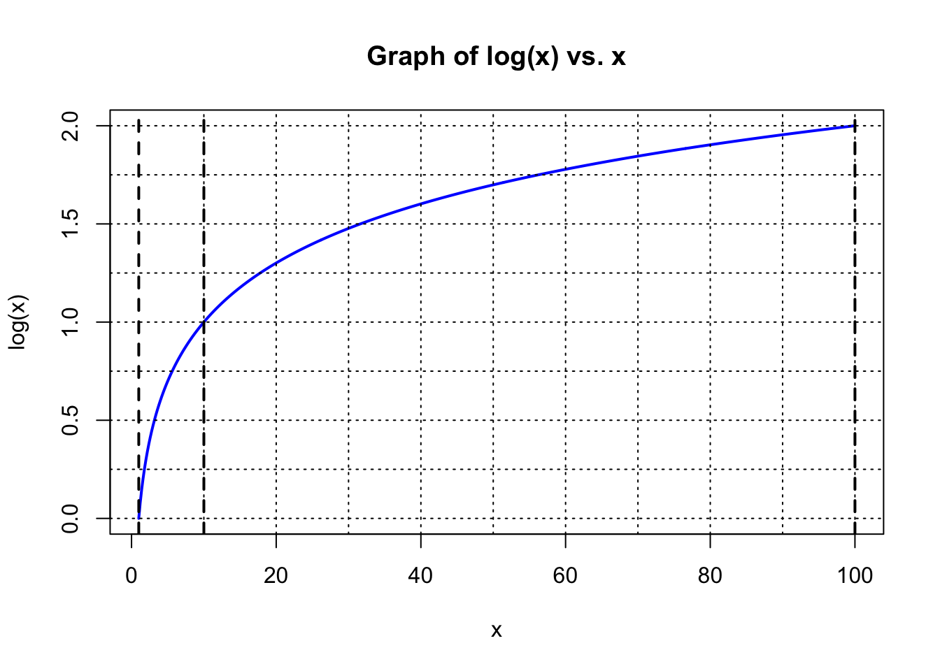
The heavy vertical dashed lines in the plot above are at values of \(x\) = \(10^0\), \(10^1\), and \(10^2\), and we see that they cross the blue curve at values of 0, 1, and 2 on the left-hand scale. Now suppose that we stretch the numerical scaling of the horizontal axis to create a linear relationship to the values of logarithms along the vertical axis. Here is the result:

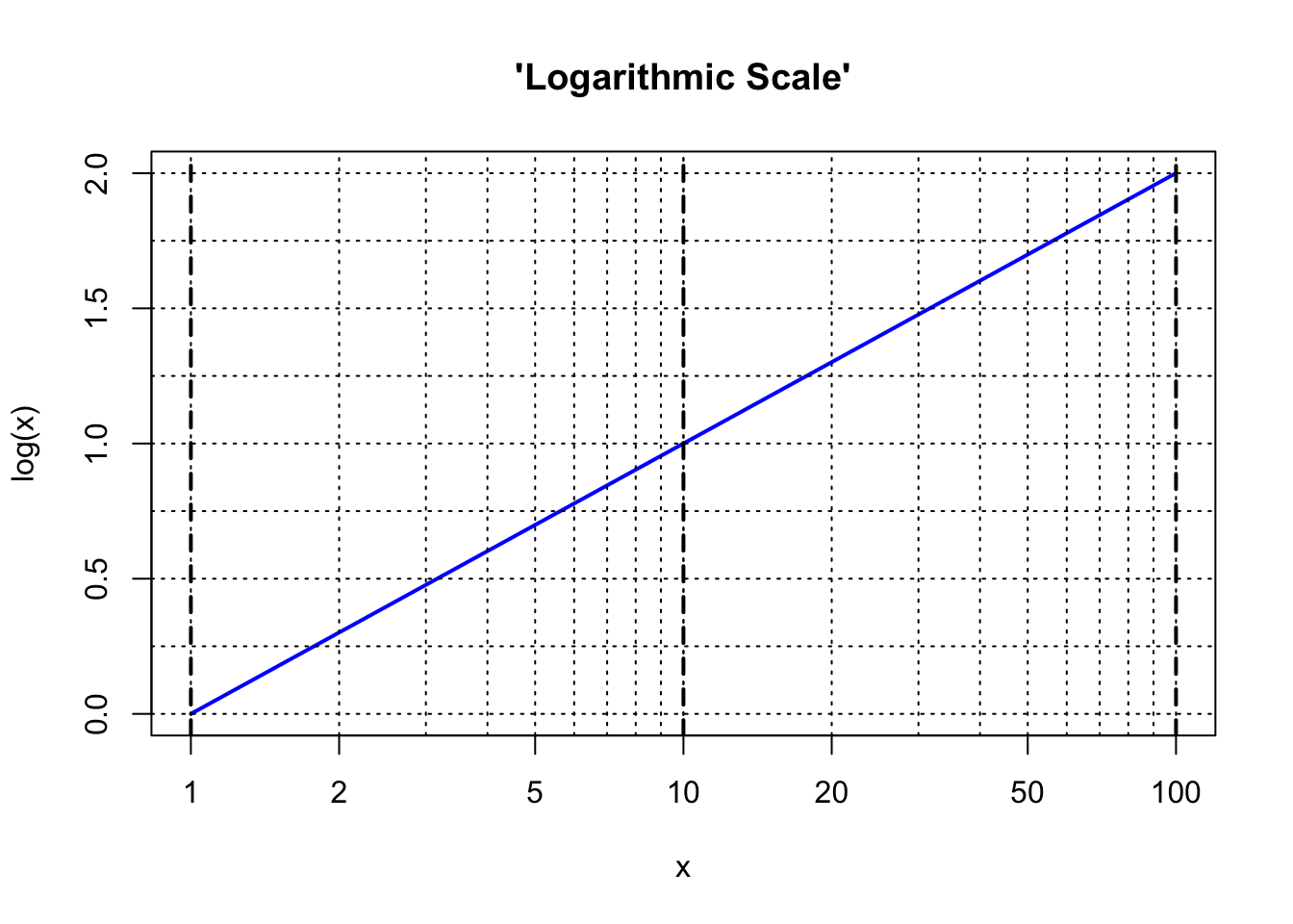
The special scaling along the \(x\) axis shown in the final figure above is often referred to as a “log scale” and this is what is found on the standard scales of a slide rule. The figure shows that with this particular scaling on the slide rule, the distance from the number 1 to the number \(x\) is directly proportional to the logarithm of the number \(x\). Notice that the distance from 1 to 10 along the horizontal axis is the same as the distance from 10 to 100 (as would be the distance between 100 and 1000 or between 0.1 and 1, and so forth). Every factor of 10 changes the logarithm by one unit. One can see also that the logarithm of 20 (distance from 1 to 20) is the same as the logarithm of 10 (distance from 1 to 10) plus the logarithm of 2 (distance from 1 to 2).

---

3. Tables de Logarithmes, Chez veuve DESAINTE, Libraire, rue du Foin, Paris, 1781.↩︎