3.7 Trigonometric Scales
Other than L, the scales discussed thus far have been simple logarithmic scales. They are used for finding products, certain powers, or certain roots of numbers. To make the slide rule more complete – particularly for the type of problems encountered in navigation, science, and engineering – scales for finding values of basic trigonometric functions were incorporated into the rules. And once again, by utilizing the logarithms of these functions, direct calculations involving trigonometric functions could be performed.
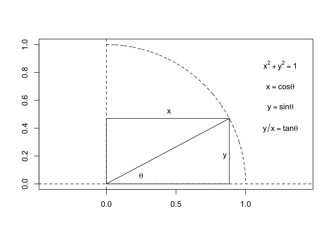
The figure below defines the basic trigonometric relationships for an angle \(\theta\) between two line segments: the sine \((\sin\theta)\), cosine \((\cos\theta)\), and tangent \((\tan\theta)\) of the angle.
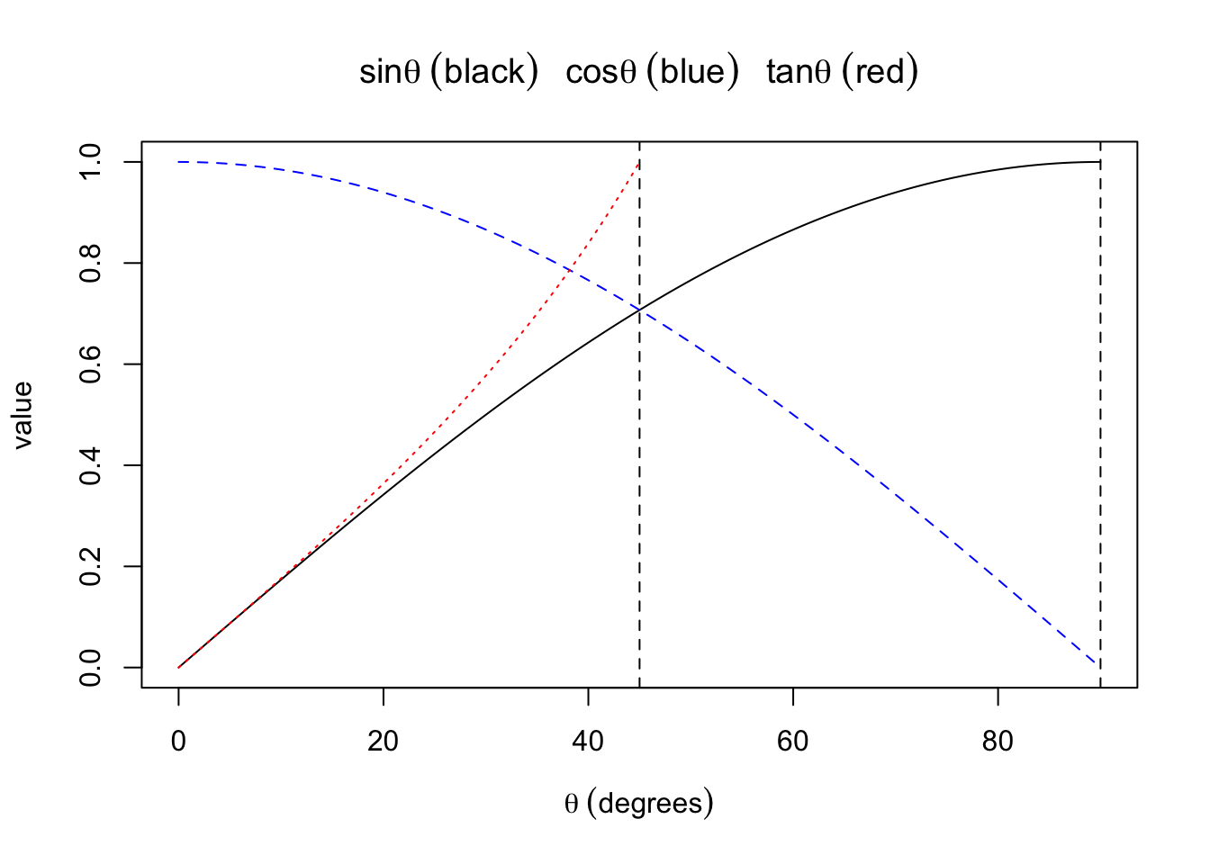
Values of these trigonometric functions for angles between zero and 90 degrees are plotted here:

The vertical dashed lines are at \(\theta\) = 45 and 90 degrees.
Scales for use in determining the sine and tangent of an angle are often found on basic slide rules. It is hard to describe all the variations of such scales in a single paragraph or subsection, as variations do exist. Suffice it to say that most scientific slide rules have a sine scale and a tangent scale of some kind and one usually can tell from their markings how to use them if one is familiar with basic trigonometry. Let’s see how such a set of scales could be implemented on a slide rule.
The values of the sine function range from 0 to 1 for angles between 0 and 90 degrees, and the values of the tangent function range from 0 to 1 for angles between 0 and 45 degrees. Consider then the C or D scale which can be interpreted to range from 0.1 to 1. By creating a new scale, usually labeled S (sine) that goes from about 5.7 degrees (because \(\sin 5.7392^\circ\) = 0.1) to 90 degrees, one can set the cursor to a certain number of degrees \(x\) on the S scale and read \(\sin x\) on the D scale, say. A separate scale – the T scale – can similarly be used to read the tangents of angles. Note that \(\tan 5.7106^\circ\) = 0.1.
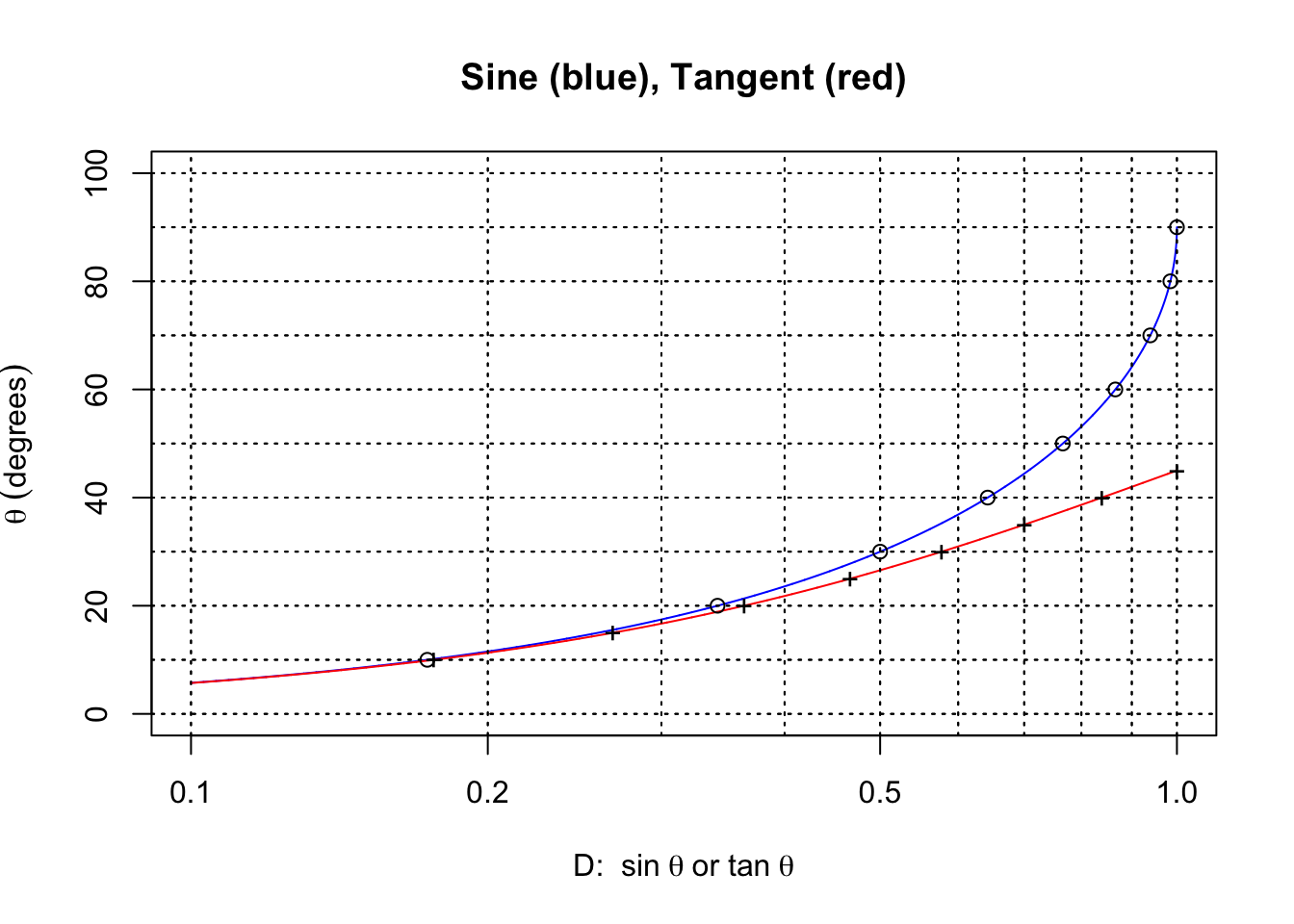
By taking the above curves for sine and tangent, exchanging the \(x\) and \(y\) axes, and plotting the \(x\)-axis with a logarithmic scaling, we get the following:
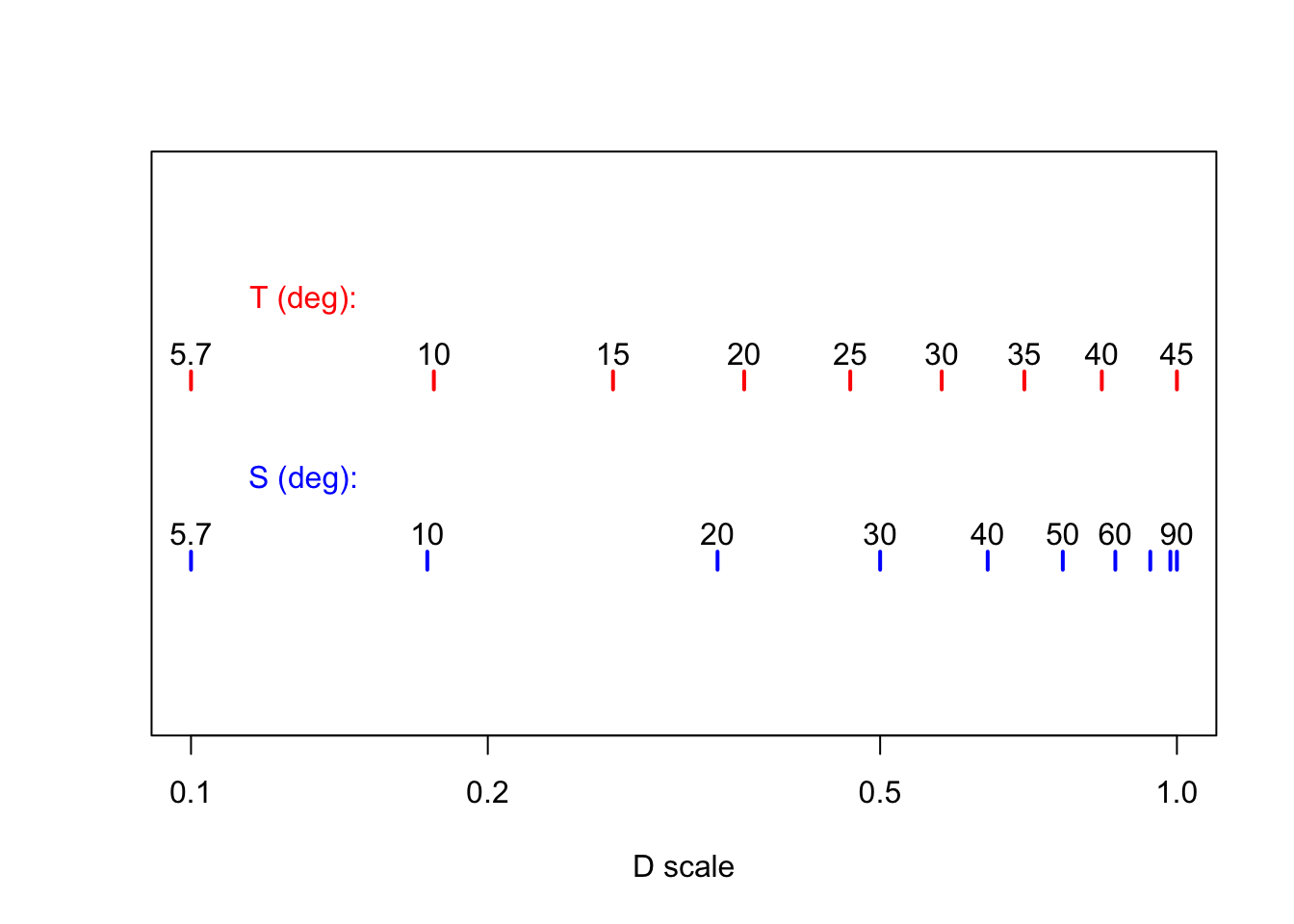
In the plot above, the circles and crosses are drawn at 10-degree intervals for the sine and 5-degree intervals for the tangent, respectively. The horizontal axis now corresponds to the D scale on the rule, and the degrees that correspond to its values are shown on the graph. These values make up the S and the T scales. As we can see, both the S and the T scales will begin at roughly 5.7\(^\circ\) and end at 90\(^\circ\) (S) or 45\(^\circ\) (T) as expected. If we take the circles and crosses and lay them out on a ruler with the spacing given above, we have created the S and T scales found on most slide rules:
Another way of thinking about these scales is to ask the following: For a certain value of \(x\) on the D scale, at what angle \(\theta\) does the sine (or tangent) have this value? In other words, we want \(x = \sin\theta\), or \(\theta = \sin^{-1}x.\) Markings for the numbers on the D (or C) scale are placed a distance \(L_0\log x\) away from the left index, where \(L_0\) is the total length of the logarithmic scale (typically 25 cm, or about 10 inches). So, numbers on the S scale will be placed a distance \(L_0\log(\sin\theta)\) from the same index, and the T scale’s markings will be \(L_0\log(\tan\theta)\) accordingly. From the earliest years of the development of the logarithm, tables of the logarithms of trigonometric functions were included in the books of logarithms because of the usefulness of these values in navigational and astronomical calculations. It is not surprising that the S and T scales were incorporated into the early Mannheim-style slide rules in addition to the standard logarithmic scales.
For angles less than about 5.7\(^\circ\), the sine and the tangent of such small angles are virtually identical. If the angles are expressed in radians, then \(\sin x\) \(\approx\) \(\tan x\) \(\approx x\). So a third scale – called ST – is sometimes found on slide rules for use with small angles. To three significant digits, \(\sin 0.573^\circ\) = \(\tan 0.573^\circ\) = 0.010. So, the ST scale has angles from about half a degree up to about 5.7 degrees, and the numbers on the D scale will need to be interpreted as between 0.01 and 0.1. The graph below shows how close the two values of sine and tangent are for small angles.
The earliest slide rules had angles marked off in degrees, minutes (1/60 of a degree) and seconds (1/60 of a minute). More modern rules used decimal degrees rather than the antiquated minutes and seconds of arc. Additionally, in the mid-1900s, the use of radians rather than degrees to describe angles became more common with many engineers and scientists. In a complete circle there will be \(360^\circ\) or \(2\pi\) radians. With decimal degrees on the ST scale, it is straightforward to convert degrees to radians and vice versa, by reading degrees on the ST scale and radians on the D scale, since for small angles \(\sin x \approx x\). To emphasize this feature many slide rule makers relabeled the ST scale as SRT, with the “R” standing for radians. Additionally, some rules can have Gauge Marks to allow for quick conversion between degrees and radians, while certain rules might even have other specific scales for conversion between these quantities or for direct readings using radians.
On some of the older slide rules, and on many “beginner’s” rules, the appropriate scales of degrees were placed on the back of the slide. On some models, by lining up the “degree” number on a line within a small window on the back of the rule the sine and tangent of that angle appears on the front of the rule, usually read off of the C scale at the end of the A or D scale. Some of the older models as well as some of the “beginner’s” rules also expect the values to be read from the A scale; when this is the case, then the entire range of \(\sin x\) from 0.01 to 1 is on the A scale, and thus interpreting a third digit is often hard.
Now if the S and T scales are on the back, the slide could be removed from the stock and re-inserted with the S and T scales facing the front of the rule, making it easier to read directly or to use directly in a calculation. Such juggling became unnecessary with the invention of “duplex” slide rules, which had a double-sided cursor and coordinated hairlines so that the scales on one side were aligned with the scales on the other side. It was common for the S and T scales to be on the slide; hence, rather than just “reading off” the values of the trig functions, one can immediately multiply or divide these values in calculations.
Up to now we have been talking about sines and tangents of angles. To find the cosine of an angle \(x\) between 0 and \(90^\circ\) (0 to \(\pi/2\) radians), \(\cos x\) = \(\sin(90^\circ-x)\) = \(\sin(\pi/2-x)\). Also, \(\cos x = \sin x/\tan x\) – an operation that can be performed rather straightforwardly. As an example, suppose we wanted the cosine of 38 degrees. If that’s all we need, we can look up the sine of 90 - 38 = 52 degrees, which is 0.788; this is the cosine of 38 degrees. Another approach would be to use the slide rule as follows:
- With the S and D scales lined up, set the cursor on the S scale to 38 degrees; the sine of this angle can be read on the D scale (if you want to know it).
- Now move the slide (not the cursor) to line up 38 degrees on the T scale at the cursor hairline.
- The cosine of 38 degrees can now be read on the D scale, directly under the 1 on the C scale.
Why does this work? Logarithms! The C/D scales are logarithmic, and so when we perform the second step above, we are dividing the tangent into the sine of the angle – and this is \(\sin\theta/\tan\theta = \cos\theta\)!
So long as the trig scales are located on the slide of the slide rule, such tricks can be used to perform many common operations. For example, suppose we want to find the hypotenuse \(c\) of a right triangle given the sides \(a\) and \(b\). For such a calculation, suppose \(b \lt a\). Then, define \(\theta\) such that \(\tan\theta = b/a\). The hypotenuse will be \(c = b/\sin\theta\). Let’s take something we know the answer to: \(a\) = 4, and \(b\) = 3. Traditionally, one might set the cursor to 4 and read, on the A scale, its square – 16 – and write that down. Then, do the same with the other number, 3 to get its square – 9. Then, add them together on paper to get 25. Next, find 25 on the A scale and read its square root – 5 on the D scale below. There are other methods for finding the hypotenuse, but here we want to do the calculation using the rule’s trig scales which are assumed to be on the slider of the rule:
- Set the cursor to the smaller number, 3 on the D scale.
- Divide by the other number, 4, by moving 4 on the C scale to line up with the cursor. Move the cursor to the end of the C scale to line up with the result (0.75).
- Reset the slide in order to look up the angle \(\theta\) on the T scale which has this tangent – you should see about 36.9 degrees.
- Now, move the S scale so that this same angle lines up with the original smaller number, 3, using the cursor.
- Looking on the D scale just below the “1” on the C scale, you should find 3 divided by the sine of our \(\theta,\) the result of which should be – say it with me – 5!
\(~~\)
Some of the advanced slide rules may have a special scale (usually called the P scale, or Pythagorean scale) that gives the value of \(\sqrt{1-x^2}\) for a given value of \(x\) on the D scale. This is a common operation for certain other computational problems, but noting that \(|\cos x|\) = \(\sqrt{1-\sin^2 x}\) means that one can use this scale to quickly find the cosine of an angle. An example of a rule with a P scale is provided here:
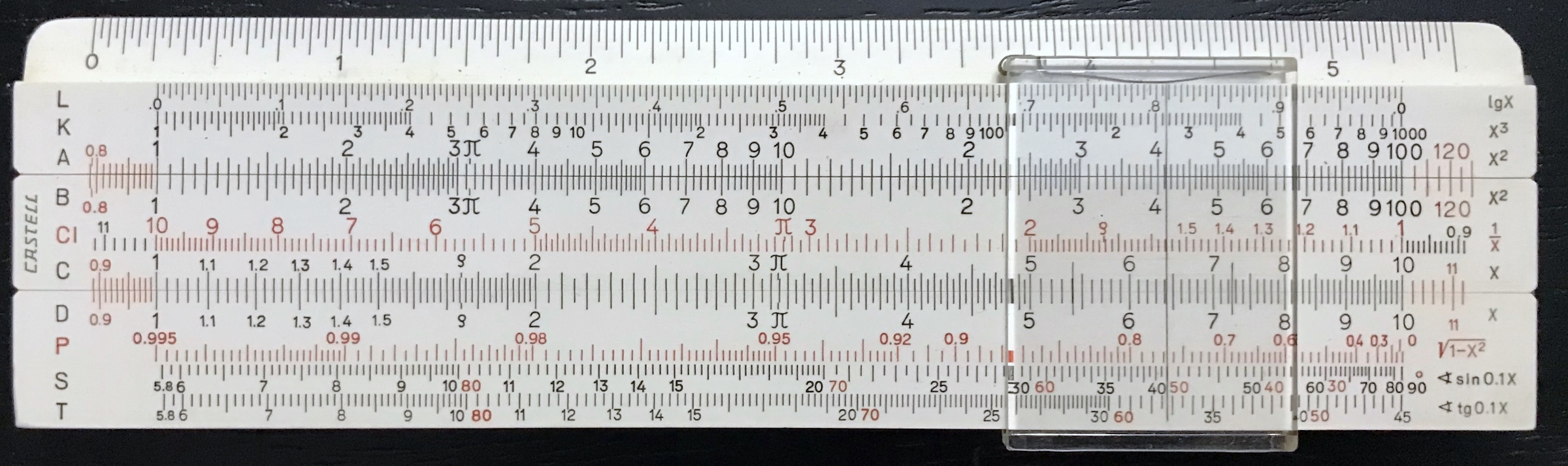
The cursor in the figure above is aligned with the 40 degree mark on the S scale. We see that the sine of this angle is 0.643 (on the D scale). On the P scale we can read off the cosine of this angle as 0.766.
Lastly, it is also important to remember that the slide rule does not take into account the “sign” of its arguments, and so as is typical of many trigonometric problems one must understand the procedures for operating in the various quadrants where angles may be greater than 90 degrees or have negative values, etc.