1.1 Exponents and Powers
Our present introduction to the logarithm continues with a review of the operation of raising a number to a power. For example, let’s continue with the simple operation of multiplying the number 2 with itself some \(p\) number of times. We call this “raising” 2 to the power of \(p\), written “\(2^p.\)” If \(p\) =2, then we say that the square of 2 , or 2 to the power 2, is \(2^2\) = \(2\times 2\) = 4. For \(p = 3\), the cube of 2, or 2 to the power 3, is \(2^3\) = \(2\times 2\times 2\) = 8. Clearly 2 to the first power (\(p=1\)) is simply \(2^1\) = 2. For completeness we must also define the operation of 2 to the power zero; if \(2^2\) is half of \(2^3\), and \(2^1\) is half of \(2^2\), then \(2^0\) is half of \(2^1.\); and half of two is just one. Thus, for \(p=0\), two to the power zero is \(2^0\) = 1. (In fact, by the same argument, any real number to the power of zero is equal to one.)
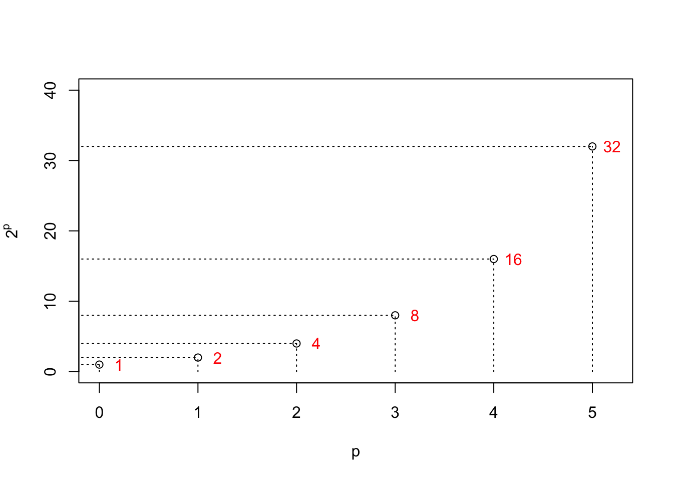
Let’s plot the results of taking \(2^p\) for the values of \(p=0,1,2,3,4,5\):
The next question is, what would be \(2\) raised to some power that is not an integer? That is, what about \(2^{0.5}?~~~~~2^{2.25}?~~~~~2^{3.659}?\) What is the meaning of such an operation? Might the results of such operations “line up” with the values plotted above?
To proceed, let’s look at a couple of properties of multiplying numbers an integer number of times. For example, take two numbers which we write as powers of 2 – call them \(2^a\) and \(2^b\). If we multiply these two numbers together we arrive at \(2^{a+b}\). For example, \[ 2^2\times 2^3 = (2\times 2)\times(2\times 2\times 2) = 2\times 2\times 2\times 2\times 2 =2^5 = 2^{2+3}. \] Additionally, if we take one of our numbers that is a power of 2 – say \(2^a\) – and raise that to another integer power – say, a value of \(b\) – the result will be \((2^a)^b = 2^{a\times b}\); for example: \[ (2^2)^3 = (2\times 2)\times(2\times 2)\times(2\times 2) = (2\times 2\times 2\times 2\times 2\times 2) = 2^6 = 2^{2\times3}. \]
In summary,
- \(c^a \times c^b = c^{a+b}\), and
- \((c^a)^b = c^{a\times b}\).
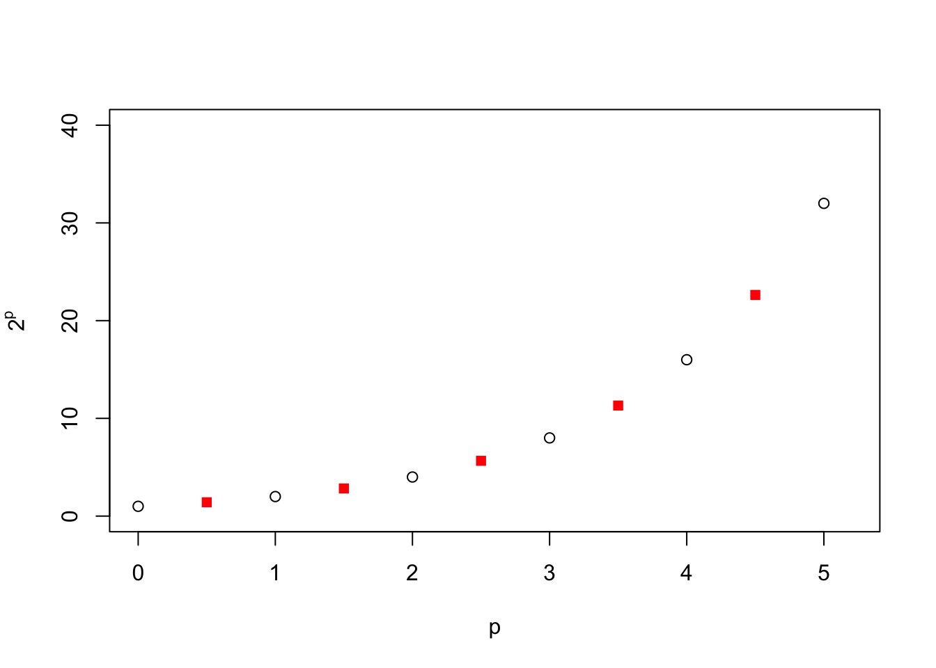
If we accept these operations as general rules, then we can determine the values of our three operations that we have asked about. First, our rules tell us that \(2^{0.5}\times 2^{0.5}\) = \(2^1\) = \(2\). Hence, \(2^{0.5}\) is the number that, when multiplied by itself, yields \(2\). We call this the square root of two, and we know its value: \(\sqrt{2} \approx\) 1.414. Thus, we can interpret \(2^{0.5} = \sqrt{2} \approx\) 1.414. Good approximations to the square roots of numbers can be found by various iterative techniques, which are often taught in Middle School mathematics classes. And now that we have a value for \(2^{0.5}\), we can see from our basic rules above that \(2^{1.5}=2\times 2^{0.5}\) and \(2^{2.5}=2^2\times 2^{0.5}\) and so forth, and so it is easy to fill in more points on our graph (red squares):
Next, what about \(2^{2.25}\)? Again using our new rules above, we see that
\[
2^{2.25} = 2^{2+0.25} = 2^2\times 2^{0.25} = 2^2\times 2^{\frac14}.
\]
We call \(2^\frac14 = \sqrt[4]{2}\) the “fourth root of 2” since, according to our rules,
\[
2^\frac14\times2^\frac14\times 2^\frac14\times2^\frac14 = 2.
\]
But through our rules of exponents we also see that \(2^\frac14\) = \((2^\frac12)^\frac12\) = \(\sqrt{\sqrt{2}}\) \(\approx\) \(\sqrt{1.414}\) \(\approx\) 1.189. Thus, finally, \(2^{2.25}\) will be \(2^2=4\) times this number, or 4.757. And, as before, knowing the value of \(2^{0.25}\), we can also easily compute \(2^{1.25} = 2\times 2^{0.25}\), \(2^{3.25} = 2^3\times 2^{0.25}\) and so forth. In addition, \(2^{0.75}\) = \(2^{0.5}\times 2^{0.25}\) = 1.6818, and thus \(2^{1.75}\) = \(2\times 2^{0.75}\), \(2^{2.75}\) = \(2^2\times 2^{0.75}\), and so forth. Now, we can fill in our plot even further (blue squares):
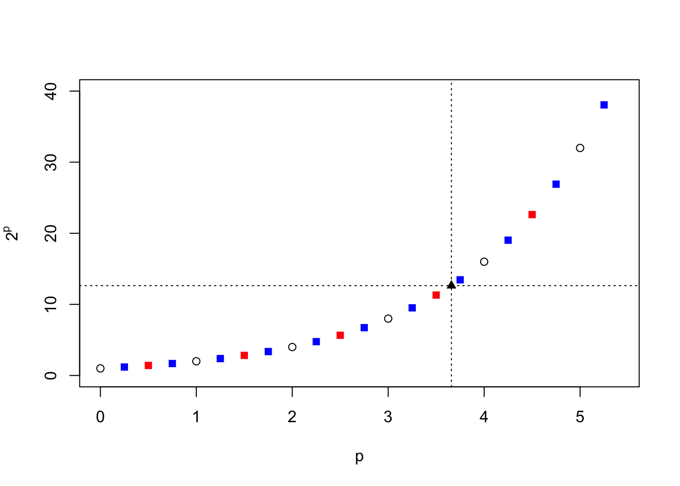
We see that the circles and the red and blue squares follow a general trend. So far we’ve been lucky to use numbers and operations (square roots) that we know well and understand. Continuing in this way, we can take further roots and powers and fill in the plot to whatever level necessary. So what about our third example, \(2^{3.659}\)? Looking at our graph above, if we follow the vertical line at \(p=3.659\) up to our group of points, we might expect \(2^{3.659}\) to have a value of about 13 or so, as read off the left-hand scale.
Following our rules above, we can write \(2^{3.659}\) as \(2^3\times2^{0.659}\) = \(8\times2^{0.659}.\) So one way (there are many) to arrive at the answer is to re-write \(2^{3.659}\) as \(2^3\times(2^{1/1000})^{659}\). But \(2^{1/1000}\) = \(((2^{1/10})^{1/10})^{1/10}\), and \(2^{1/10}\) = \((2^{1/5})^{1/2}\). Hence,
\[ 2^{3.659} = 2^3 \times \left[ (((((2^{1/5})^{1/2})^{1/5})^{1/2})^{1/5})^{1/2}\right]^{659} = 2^3 \times \left[\sqrt{(\sqrt{(\sqrt{2^{1/5}})^{1/5}})^{1/5}}\right]^{659}. \]
If we are able to find the fifth root of a number, as well as the square root of a number, then we can compute \(2^{3.659}\). That is, we can find the fifth root of 2 and take the square root of this result. Then take this answer and repeat the process two more times. Finally, we take this result, multiply it with itself 658 times, and end by multiplying by 8. This might take quite awhile by hand, but can be done easily on a modern personal computer:
## [1] (2^3)*(sqrt(sqrt(sqrt(2^(1/5) )^(1/5) )^(1/5) )^659) = 12.6319021872098The value of \(2^{3.659}\) =12.6319 is included on our plot above as a black diamond and, again, falls into the pattern of our other computations. If we continue in this vein, in principle we could fill in an entire curve and hence for any chosen value of \(p\), integer or non-integer, we can compute a value for the operation \(2^p\) to some desired accuracy.
Empowered with this new information, problems now can be posed in reverse. We can imagine filling in our graph until a continuous curve appears, and then take this curve and switch the axes as shown below. The point of this switching of the axes is to emphasize that any number \(x\) can be represented by the number 2 raised to a particular power \(p\):
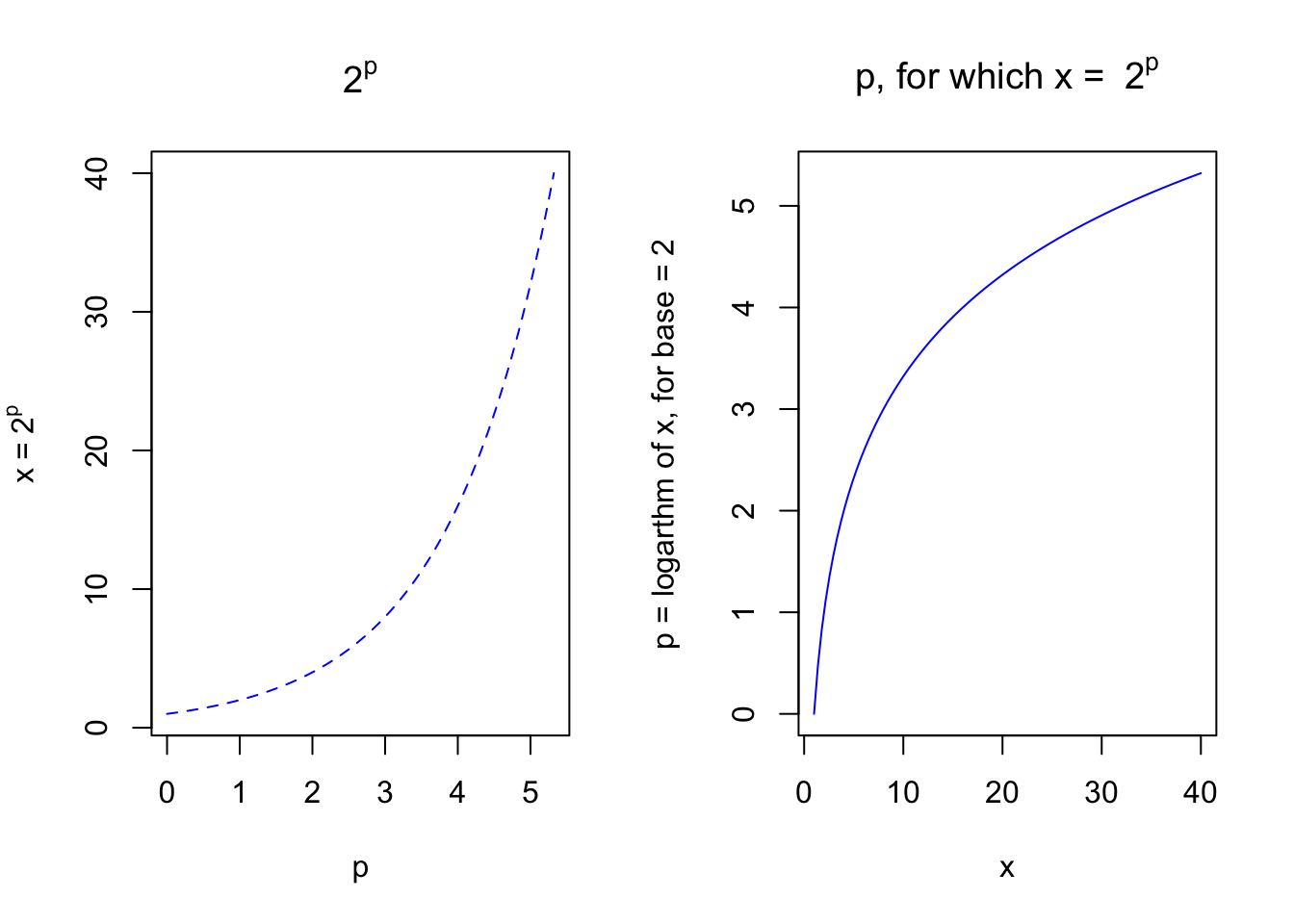
The concept of a logarithm is to chose a base (\(2\), in our example here) and ask the question, “Given a general number \(x\), to what power must we raise the base in order to obtain this number?” The answer – the exponent \(p\) – is called the logarithm of \(x\) for that particular base. Although we used \(2\) as our base number above, the choice of “2” is arbitrary. The same procedures could be used for any base we choose such as 3 or 10, and includes the use of non-integers or even irrational numbers such as \(\pi\) = 3.141592… The only caveats at the moment are that the base number be greater than zero (zero raised to any power is zero; and negative numbers complicate things) and it cannot be one. (One raised to any power is just one.)
So why go through all of the trouble of finding logarithms? Suppose one wanted to multiply two multi-digit numbers, \(x\) and \(y\). Multiplying two numbers such as \(x\) = 28718 and \(y\) = 81793 could take quite a while and be prone to errors if not performed very carefully. With a table of values of logarithms for our chosen base (here, base = 2), we can look up the values of the logarithms \(p\) and \(q\) for the numbers \(x\) and \(y\) that satisfy \(x = 2^p\) and \(y = 2^q\). Next, we reason that \(x\times y\) = \(2^{p+q}\). While multiplying the numbers \(x\) and \(y\) may take take awhile by hand, the summation of \(p\) and \(q\) can be performed much more quickly and easily (and, typically, with much less chance for error). We then look in our table for the number that has the total of \(p+q\) as its logarithm, and this would be our final answer for \(x\times y.\)
The realization that the multiplication of numbers can be equated to the addition of so-called logarithms was Napier’s major achievement. If logarithms of real numbers could be tabulated to sufficient accuracy, then complicated multiplication and division problems could be reduced to much simpler addition and subtraction calculations. In Napier’s day, this was particularly important in navigation calculations performed at sea, for instance. Now, such calculations could be performed much more quickly and accurately. One didn’t need to spend large amounts of time multiplying large numbers long-hand using pen and paper. Rather, logarithms could be looked up in a book of numerical tables and added together to get a result. Napier and his English colleague, Henry Briggs, produced detailed tables of common logarithms within just a few years of their mathematical development. And the ability – even in the 1600’s – to compute the values of logarithms of numbers to sufficient accuracy led almost immediately to the invention of the slide rule. A systematic procedure for calculating the logarithm of an arbitrary number is left to the next chapter. Meanwhile, in the remaining sections of the present chapter, we will assume that values of logarithms are available to us as we investigate their various properties and explore their use in performing basic calculations.