8.10 Power Rules
Many problems in science, engineering, and even in business applications, require raising numbers to powers. Common examples include the calculation of loan payments or account growth given a certain interest rate. A simple 5 percent interest rate per year would increase a principal amount by a factor of \(1.05^5\) after five years. While this might be easy to compute on paper, a calculation after 25 years – \(1.05^{25}\) – might demand a slightly different approach.
Exponential growth and decay calculations, such as might be found in electrical and electronics evaluations, radioactive decay, or in the growth of cases during a pandemic situation – problems of the form \(N = N_0\;e^{k\cdot t}\) – involve raising a number \((e)\) to a power \((k\cdot t)\).
Sometimes values of complicated functions can be estimated by a process called a power series expansion in which values of the function can be expressed in terms of a series of terms where the independent variable \(x\) is raised to a series of powers. As an example, the function
\[ f(x) = \frac{x^2}{4-x^2} \] can be expressed as a power series so long as \(|x|<2\). This series is an infinite sum of terms given by the formula \[ f(x) = \frac{x^2}{4-x^2} = \frac{x^2}{4} + \frac{x^4}{4^2} + \frac{x^6}{4^3} + \ldots \] Hence, to evaluate the value of \(f(1.05)\), for example, one can take 1.05 and raise it to the powers indicated, dividing each term by the appropriate number of “4”s and then summing up the results to get a final value within a desired accuracy. Many problems in science and engineering, particularly ones involving quite complicated functions, can be solved using power series and then evaluated numerically in this way.
8.10.1 The Power of Logarithms
As described in our chapter on Computing Logarithms, the logarithm of a number is just the power to which a base number must be raised in order to arrive at the number in question. Hence, logarithms – and log scales – are intricately related to raising numbers to powers.
Suppose we wish to take a number to a power, such as \(2.33^5\). We can use the C, D, and L scales on a slide rule (and perhaps a pen and paper) for the task. We know that \(\log x^r\) = \(r\log x\), and so the procedure is to note that \[ \log x^r = r\cdot \log x = 5\cdot\log(2.33) . \] Setting the cursor to 2.33 on the D scale we can find the log of 2.33 on the L scale: 0.367. The cursor is then moved to this number on the D scale, and then multiplied by 5 using the C scale. The result should be roughly 1.837, though the last digit may be hard to determine accurately on the slide rule. As this result is equal to 0.837+1, we need to find the number whose logarithm is 0.837 and multiply this result by 10 (due to the “+1”). Lining up the cursor with 0.837 on the L scale, the number with this logarithm is 6.87. So finally, after multiplying by 10, we find that \(2.33^5\) = 68.7. For comparison, using the computer to compute the answer we get \(2.33^5\) = 68.672. Note, however, that if we had only used 1.84 in our earlier step, because perhaps that is all the accuracy we have with the slide rule at hand, then we might arrive at a result of 69.1 or so. So our calculation with all of its steps is accurate to perhaps a few percent.
The early Mannheim style slide rules had C/D and A/B scales and often times on the back side of the slide were S, T (sine and tangent) and L (log) scales. Raising a number to a power in the way described above was a common use of the L scale.
8.10.2 Roget’s Log-Log Scale
Interestingly, in 1814 Peter Mark Roget, M.D. – yes, the same Roget of the famous “Roget’s Thesaurus” – wrote a paper which was delivered subsequently to the Royal Society in England in which he described a new “log-log” slide rule scale. The argument goes along these lines:
Suppose \(y = x^r\). Then,
\[ \log y =\log x^r = r \log x \] as was just described; but taking the logarithm again of each side, we get \[ \log \log y = \log r + \log \log x. \]
Since the standard slide rule already has scales (C/D) with logarithmic lengths (the “\(\log r\)” portion of the above), then one only needs scales that vary as \(\log\log x\) on the rule to which one adds values of \(\log r\) in order to quickly ascertain the value of a number raised to an arbitrary power.
One year later in 1815, Roget was himself elected a Fellow of the Royal Society; his paper was published in the Society’s Philosophical Transactions that same year.27
Though there are a few early examples of individual slide rules with log-log scales, this application on the slide rule appears to have been lost for a while, surfacing again after about 90 years, as the need for such calculations began to increase.28 Between 1900 and 1909 the makers Dennert and Pape in Germany and Keuffel and Esser in the United States began manufacturing slide rules with log-log scales for use in the complex engineering and scientific calculations of the day.
8.10.3 Creating a Log-Log Scale
The standard C/D scales on a slide rule are marked with numbers in the range 1 \(<r<\) 10 in logarithmic fashion, where the distance from 1 is proportional to the common logarithm of the number, \(\log r\). The C/D scales go from 1 to 10 because log 1 = 0 and log 10 = 1. Using our earlier notation, we want a log-log scale to also have a range of values of 0 to 1, so that we can add “\(\log r\)” to “\(\log \log x\)” in our calculation. Since 0 = \(\log \log 10\), and 1 = \(\log \log 10^{10}\), this is a scale range that we could use for our purpose. Thus, on this scale, the range of values of \(x\) would go from 10 to \(10^{10}\). To raise numbers to powers, we use the C scale on the slide to “add” values of \(\log r\) to values of \(\log \log x\) found on the stock of the slide rule. Suppose the C scale has a length of 10 inches from 1 to 10. We start our “Log Log” scale with a value of 10. Then the distance from the left index over to a general number \(x\) will be equal to (10 inches)\(\cdot\log \log x\).
Below is an image of a Pickett Model 4 slide rule from the Collection. The back side of the rule has a scale labeled LL4 which fulfills the requirements just outlined. The image shows the beginning and end of the LL4 scale, which ranges between 10 and \(10^{10}\). The image also shows the C/D scales which run from 1 to 10.
 |
 |
| LL4 starting at “10” | LL4 ending at “\(10^{10}\)” |
As an example, let’s use this scale to find the value for \(12^{2.7}\). In the image below, we see that the index of the C scale is set at 12 on the LL4 scale. Moving the cursor to 2.7 on the C scale, we can read the result under the cursor on the LL4 scale: 820. (By computer: \(12^{2.7}\) = 819.954.)
 |
 |
| C index at 12 on LL4 | result on LL4 under “2.7” on C |
8.10.4 Mixed-Base Log-Log Scales
The Pickett example above has log-log scales based on the common logarithm. However, it was realized very early on that using a mix of common and natural logarithms can perform the same calculation, but also has other advantages.
If we want to compute \(y = x^r\), we can first find the natural log of both sides, and then take the common log of the results:
\[ y = x^r \\ \ln y =\ln x^r = r \ln x \\ \log \ln y = \log r + \log \ln x \] Again the C scale can be used to add “\(\log r\)” to values of \(\log\ln x\) to find the value of \(y\).
Note that 0 = \(\log \ln e\), and 1 = \(\log \ln e^{10}\); so, this, too, is a scale range that we could use to raise numbers to powers using the C scale on the slide. This scale would start at \(e^1\) = 2.718 and would have a maximum extent of \(e^{10}\) \(\approx\) 22000. While this is a much shorter range than for the Base 10 log-log scales, it should cover most of the needs of everyday problems, and one should expect more accuracy in the results for slide rules of the same physical length. In either case, whether base 10 log-log scales are used or mixed base log-ln scales are used, these are all referred to as “Log-Log” scales. They are most frequently labeled “LL” (LL1, LL2, etc.), though other labels are often found such as “Ln”, “ln”, etc. Some of the early Pickett models used N1, N2, etc., for their scale names, especially for the totally Base-10 systems.
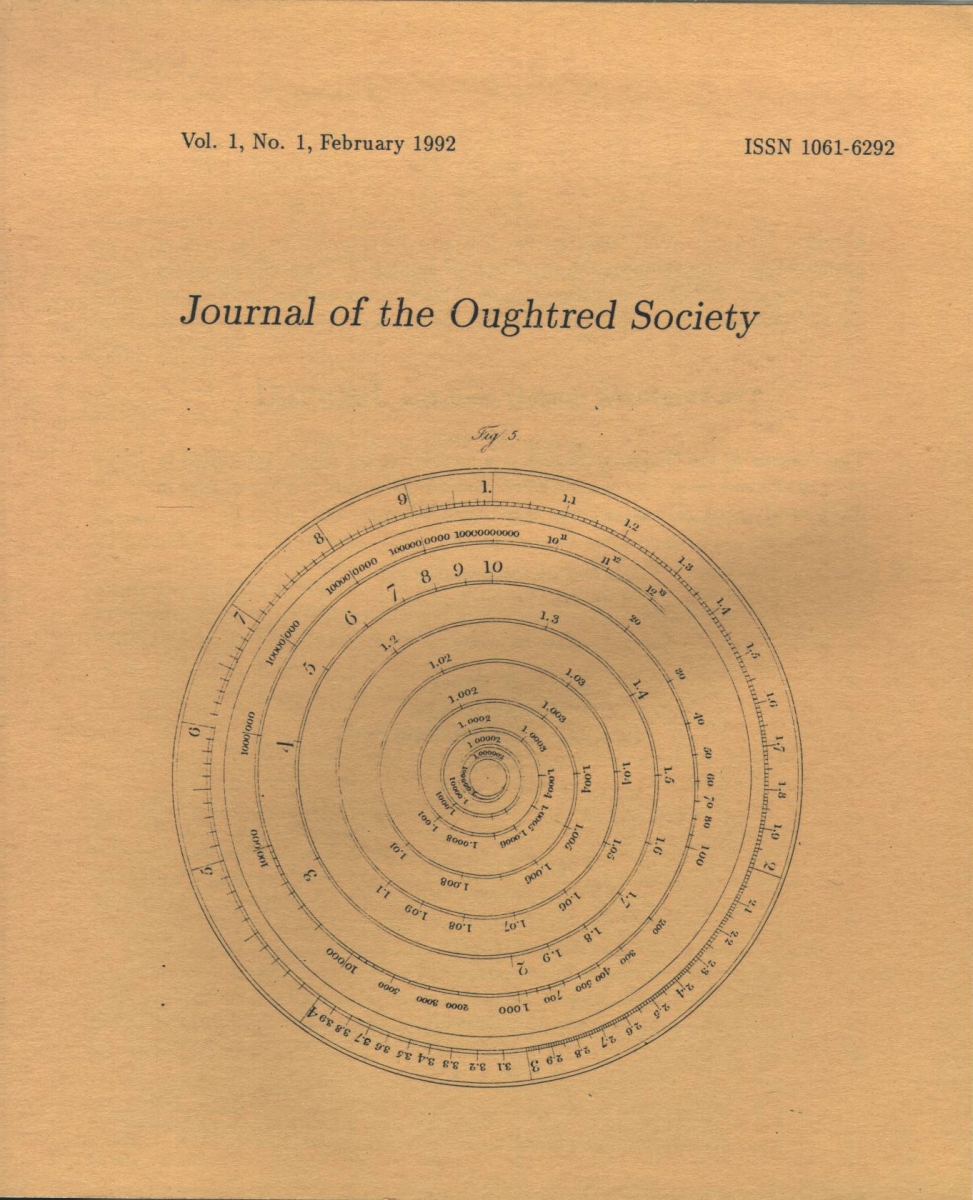
When Roget introduced his concept in 1815, his article, ““Description of a new instrument for performing mechanically the involution and evolution of numbers”, included an illustration of a circular slide rule for raising arbitrary numbers to arbitrary powers. An image of this device was on the cover of Issue 1.1 of the Journal of the Oughtred Society, and is reproduced below. From this figure it is easy to confirm that his system was “log log” system rather than a “log ln” system, or made from other combinations of bases. However, when log-log slide rules began to appear near the turn of that century, other bases were sometimes employed. If we have Base 10 scales such as C and D on the slide rule, then the log-log scales could be in any base, since we can write
\[ y = x^r \\ \log_a y =\log_a x^r = r \log_a x \\ \log \log_a y = \log r + \log \log_a x \]
for any base \(a\). Slide rules from the early 1900s are known to have be made using bases of \(a\) = 2, 10, and one with a base near 3 made by Faber.29 It was in 1909 when Keuffel and Esser introduced their Model 4092 Log Log slide rule where \(e\) = 2.71828 … was first used as the base \(a.\) This quickly became the standard in the industry, though some slide rule makers – Pickett in particular – continued to use \(a\) = 10 on several of their models.
8.10.5 Segmented Log-Log Scales
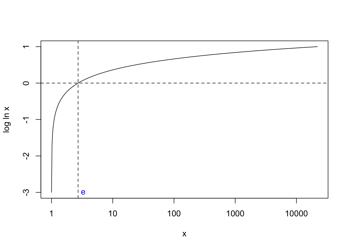
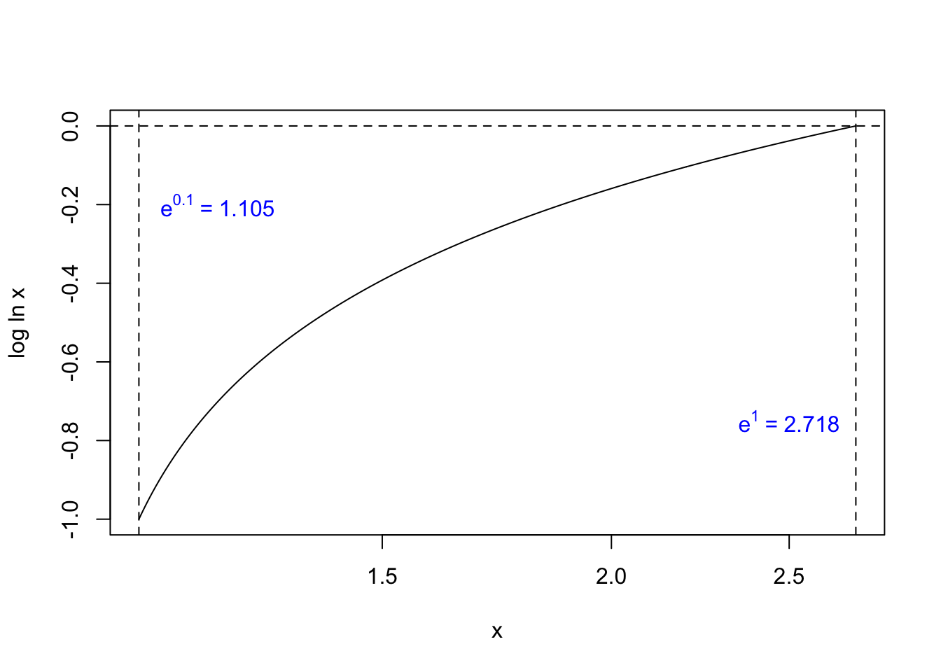
As can be seen in our plot above, for numbers less than \(e\), the natural logarithm will less than one, and the common log of that number will be negative. But this doesn’t prevent one from extending the log-ln scale to the left. From \(x\) = \(e\) to \(x\) = 22000, the vertical scale varies from 0 to about 1. That is, the \(\log\) of \(\ln x\) changes by 1 (\(\ln x\) changes by a factor of 10). We can extend our slide rule log-log scales to the left by continuing to re-interpret the range on the C/D scale through lower decades. If we interpret the ends to be at 0.1 and 1 on the C/D scale instead of 1 and 10, then the two ends of the new log-log scale would represent values of \(\log\ln e^{0.1}\) and \(\log\ln e^1\). Here is a plot of this function across this range:

Continuing, between \(\log\ln e^{0.01}\) and \(\log\ln e^{0.1},\) the value of \(\log\ln x\) changes by another unit \((\ln x\) changes by another factor of 10):
So to summarize, to produce our first mixed-base log-ln scale, we need a range between \(e^1\) = 2.72 and \(e^{10}\) = 22026 which lines up with the C/D scales that vary between 1 and 10. Again, it’s always good to check: \(\log\ln e^1\) = \(\log 1\) = 0; \(\log\ln e^{10}\) = \(\log 10\) = 1, thus providing the same linear distance across the slide rule as on the C/D scales. In the same spirit, if our C/D scales are taken to be in the range of 0.1 to 1, then we can create a log-log scale that ranges between \(e^{0.1}\) = 1.105 and \(e^1\) = 2.72. Creating a separate scale on the slide rule for each decade of C-scale values – 1 to 10, 0.1 to 1, 0.01 to 0.1, and so on – our 10 inch rule can cover a large range of log-ln values. The table below shows the end values of the four most common scales found on such log-log slide rules:
| Scale | left limit | right limit | |
|---|---|---|---|
| D | \(x\) | 1 | 10 |
| LL0 | \(e^{x/1000}\) | 1.001 | 1.0101 |
| LL1 | \(e^{x/100}\) | 1.0101 | 1.1052 |
| LL2 | \(e^{x/10}\) | 1.1052 | 2.7183 |
| LL3 | \(e^{x}\) | 2.7183 | 22026 |
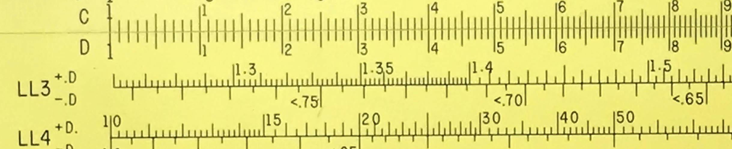
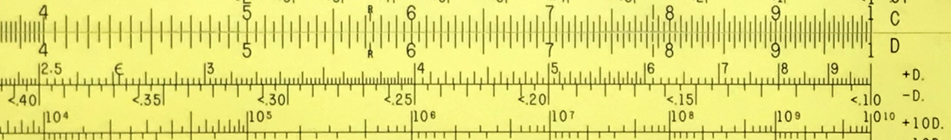
The magic of logarithmic scales allows for not only taking everyday numbers to relatively low powers (like, taking \(3^{3.6}\)), but also for taking smaller numbers – close to one – to much larger powers (like, taking \(1.02^{32}\)). In the first example, a single scale is used – LL3 – in conjunction with the C scale, provided that the result is less than about 22,000. In the second case, it is easy to find 1.02 on the LL1 scale, line up the index of C to this, and then move the cursor to “3.2” on the C scale. The result below the cursor on the LL1 scale – 1.0654 – is actually \(1.02^{3.2}\). But since the various LL scales differ by a “decade” in value of \(\ln x\), then \(1.02^{32}\) is found on the next scale up, in this case on the LL2 scale. Here, we read the correct answer: \(1.02^{32}\) = 1.885. On the LL3 scale we can read \(1.02^{320}\approx\) 560. (More accurately, by computer: 565.01.)
In about 1900, Dennert and Pape began manufacturing their first log-log slide rule and produced another version in about 1908.30 Then, in 1909, K&E introduced their first log-log rule, the Model 4092. This first version – an example of which is shown below from the Collection – had three scales labeled LL1, LL2, and LL3. From the end point values we can see that they are “log-ln” scales. And the “LL” labels became standard for many future slide rules containing these scales.
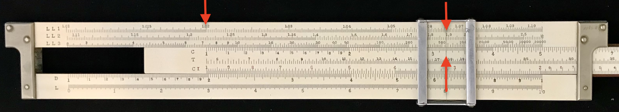
Here is a setting of the K&E 4092 taking \(1.02^{32}\) using the LL1, LL2, and C scales:
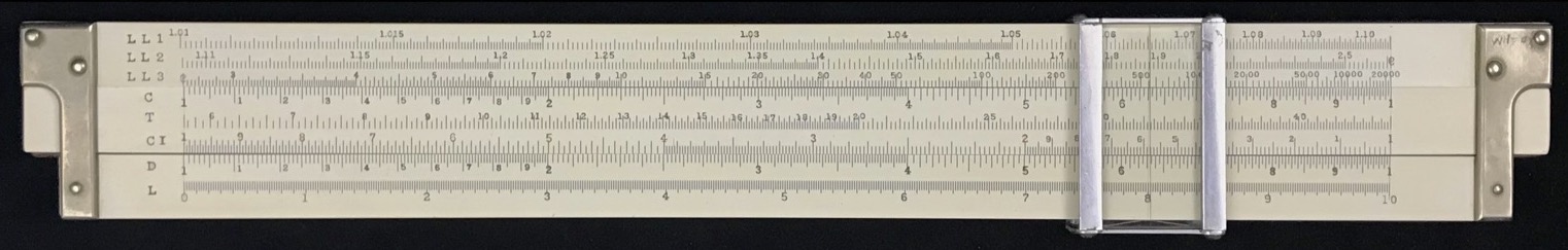
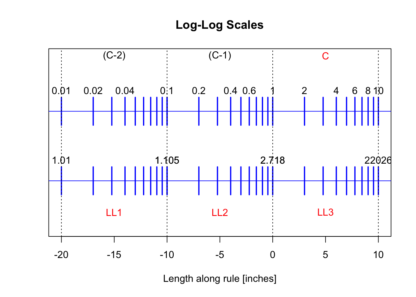
To emphasize the approach, one can imagine a very long rule, say 30 inches in length, with three decades worth of “C/D” scales, as shown below:

Below the C scale is the “log-log” scale. The sections that represent the standard LL1, LL2, and LL3 scales are indicated. The “1” index of the C scale is aligned with the “e = 2.718” mark on our log-log scale in the above image.
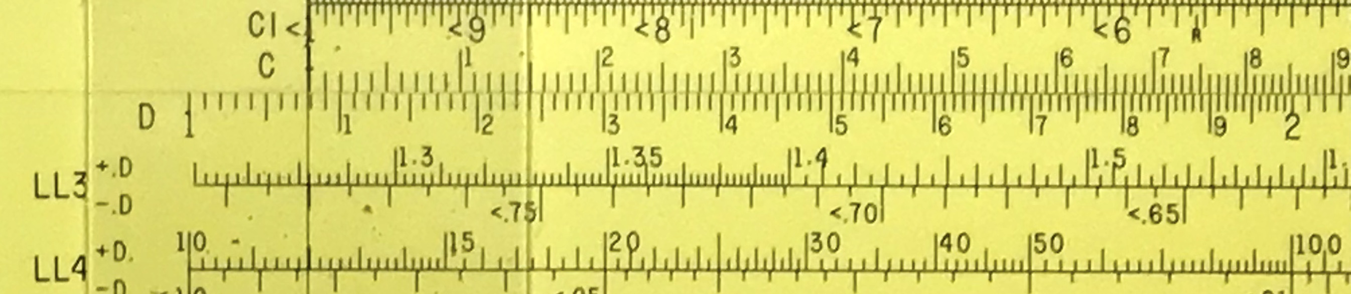
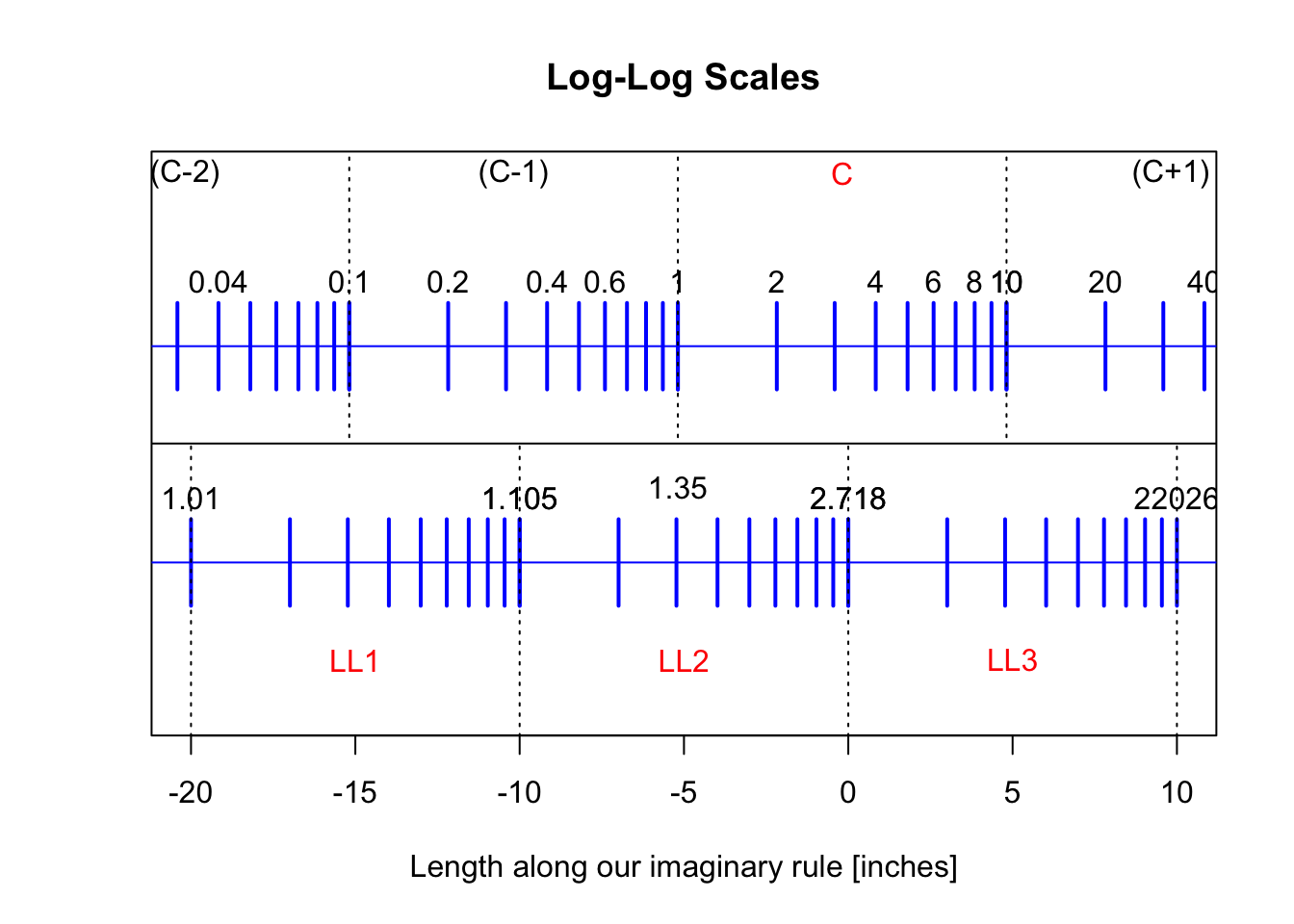
Now suppose we wanted to take the number 1.35 and raise it to the fourth power. Notice that 1.35 falls on the LL2 scale. If we slide the C scale to align the “1” with 1.35, as is shown below, we see that the “4” on the C scale is beyond the boundary of the LL2 scale off to the right:
In fact, the answer – 3.32 – falls in the LL3 region. So, to actually arrive at this answer in the “real world”, we re-index the slide to the left31 to get the “4” mark back on scale, and then look at the LL3 scale for the answer.
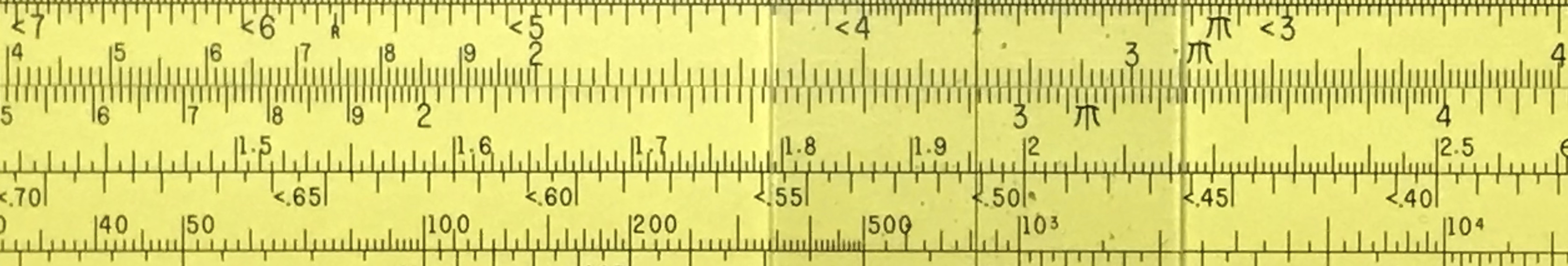
Also notice where one would find 1.35 raised to the 0.4 power, or to the 0.04 power – the answers lie at the “4” mark on C, as shown below, but in the LL2 and LL1 scales after proper re-indexing:
And, of course, raising 1.35 to the 40th power would be totally off-scale to the right. By “re-interpreting” the C scale as shown, the LL1,2,3 scales on the slide rule are equivalent to having a single 30-inch log-log scale.
8.10.6 Reciprocal Log-Log Scales
Now a number less than one will have a natural logarithm that is negative and hence its common logarithm will be undefined. So how do we deal with raising such numbers to arbitrary powers? The reciprocal of a number less than one will be a number greater than one. If \(x<1\) then \(1/x>1\). A number raised to a negative power is simply the reciprocal of the number raised to the corresponding positive power: \(x^{-r} = 1/x^r\). Hence finding a number raised to a negative power can be performed by finding \(x^r\), say, using the log-log and C scales as described above, and then finding that result on the C scale in order to use the CI scale (typically included on such log-log slide rules) to find the inverse. This complicated procedure was simplified by the introduction of log-log scales for negative exponents or reciprocal scales, namely LL01 = 1/LL1, LL02 = 1/LL2, and so on. These scales are used in the exact same way as the original log-log scales. But note that a number less than one when raised to a power greater than one will result in a smaller number; hence, these scales decrease to the right. The table below shows the values found on these scales at the end points of the standard D/C scales:
| Scale | left limit | right limit | |
|---|---|---|---|
| D | x | 1 | 10 |
| LL00 | \(e^{-x/1000}\) | 0.999 | 0.99 |
| LL01 | \(e^{-x/100}\) | 0.99 | 0.9048 |
| LL02 | \(e^{-x/10}\) | 0.9048 | 0.3679 |
| LL03 | \(e^{-x}\) | 0.3679 | 5e-05 |
The addition of these scales on the slide rule has several benefits. First, raising numbers to negative powers can be done with one setting of the cursor, rather than several settings and transcriptions as described previously. Secondly, with both LL and inverse LL scales, values of \(e^x\) and \(e^{-x}\) can both be read with a single setting of the cursor, allowing one to more quickly compute the values of hyperbolic functions such as \(\sinh x\) = \((e^x-e^{-x})/2\).
One can also use the mixed-base log-log scales to find the natural logarithms of numbers, since for \(y=e^x\), we have \(x=\ln y\). These features in conjunction with the original use for finding arbitrary numbers raised to arbitrary powers make the mixed-base log-log scale sets extremely versatile and valuable.
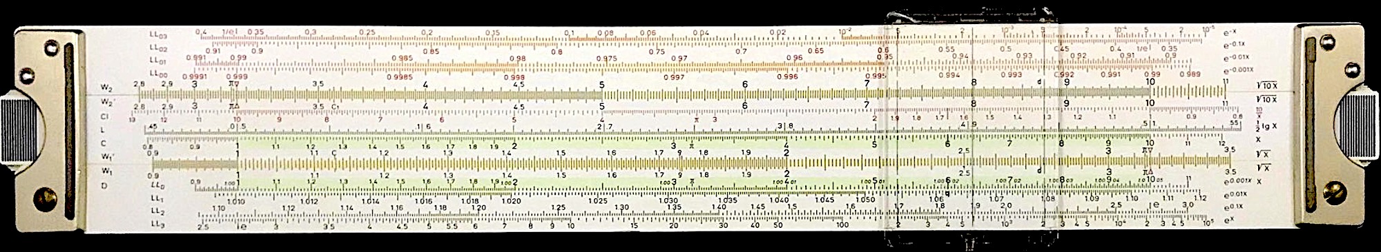
Below is an image of a Faber-Castell Model 2/83N showing the full complement of 8 LL scales all on one side of the slide rule:
8.10.7 Examples of Circular Log-Log Scales
Besides the LL scales found on standard linear slide rules, many circular slide rules also have LL scales. Circular slide rules tend to have a C scale that wraps once around the circumference. Hence, a single rotation of the cursor is a multiplication of 10. The LL scales can thus be established by each being a complete circle as well, enumerated with proper end limits according to our rules above.
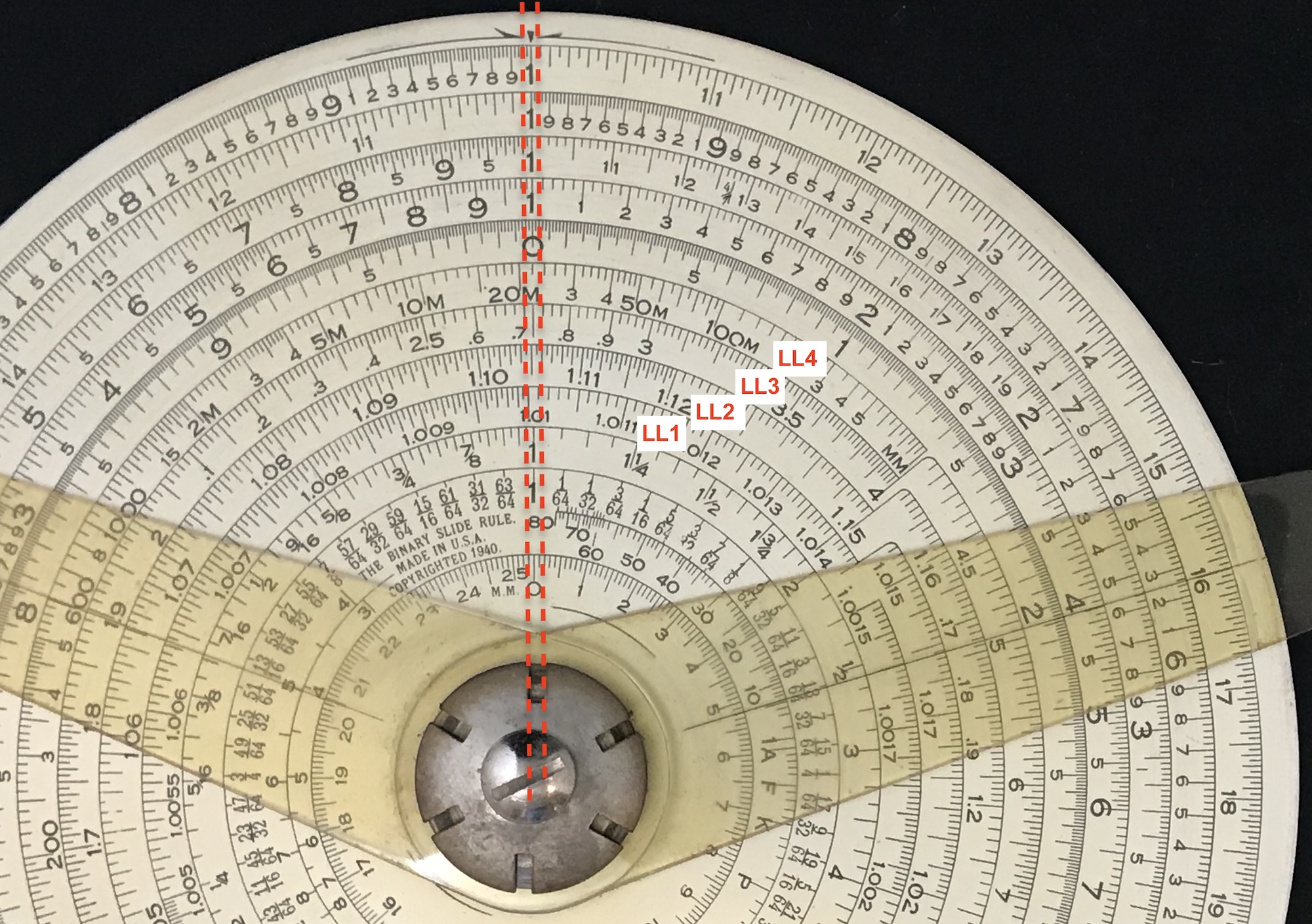
The left image below shows a Gilson Binary circular slide rule which has LL scales. The scales are all printed on a single surface, and one can see that the index (the “1”) of the C scale, A scale, etc. all line up. The four LL scales are marked in the image, and we see that the values on these scales as they pass the index are at values of about 1.01, 1.105, 2.74, and 22000. (On this scale, “20M” refers to 20,000.) Looking closely at these scales, just to the left of the cursor on the right side of the image, you can see that these scales abruptly change from one to the next level up. Each scale is an actual circle, and the total span goes from 1.0015 to 1 million (MM).
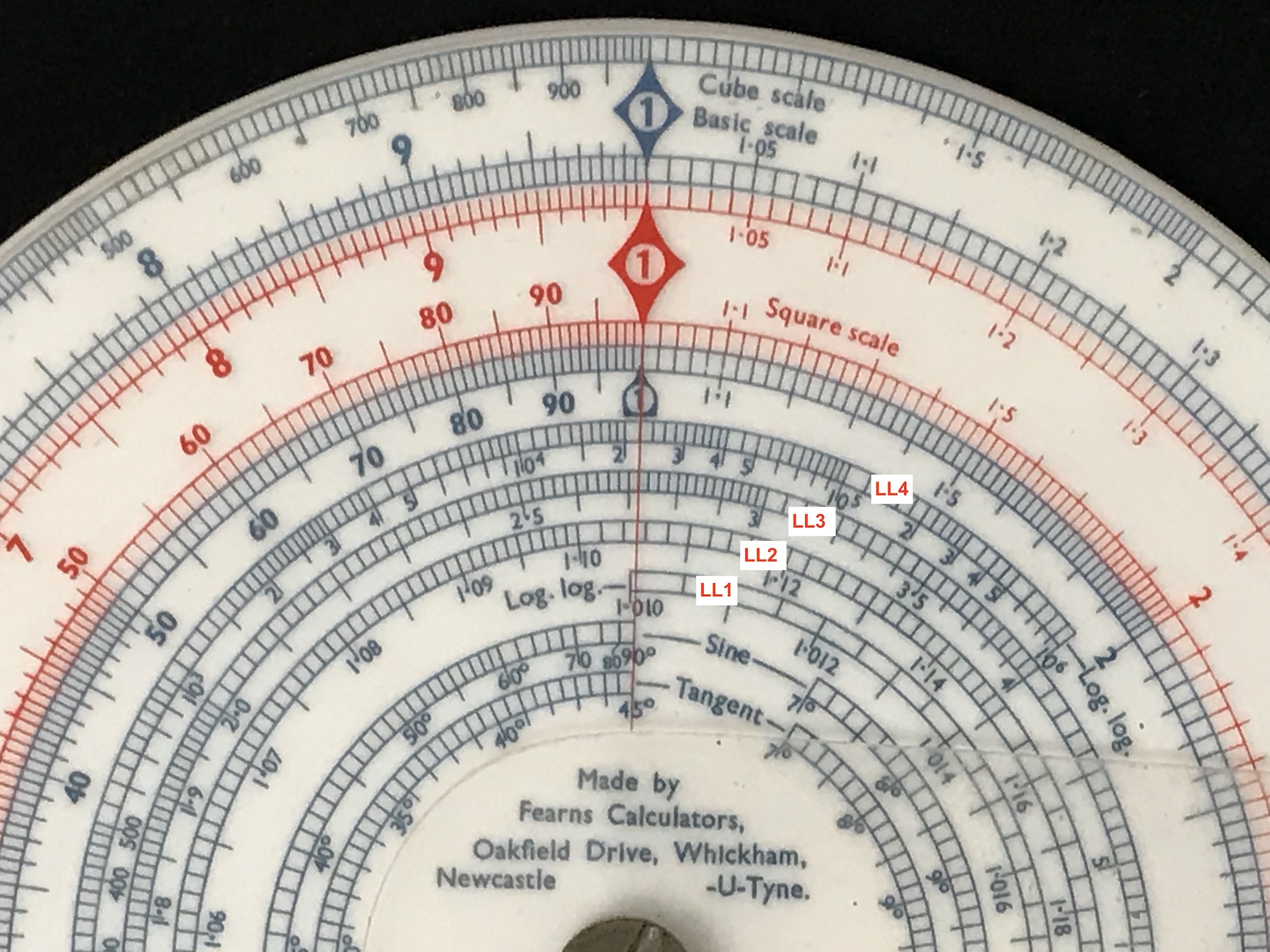
There are also examples of true “spiral” scales applied to circular slide rules, where a single continuous scale has been produced, just as was envisioned by Roget 209 years ago. One example, shown in the right image below, is the Fearns Calculators Model A13. Looking along the line of indices, one can see the starting point of the spiral, labeled “Log.log.”, at a value of 1.010. The spiral passes the indices at the usual values and, again, ends at a value of 1 million. The labels “LL1, LL2, …” in the image are there just to show relevant portions of the spiral. As stated, the scale is actually just one single continuous curve.
 |
 |
| LL scales on the Gilson Binary | Spiral LL scale on Fearns A13 |
8.10.8 Applications and Examples
The best way to become better acquainted with log-log scales is, of course, to use them. Below are some simple problems which can be solved using the LL scales. I used the Faber-Castell slide rule 2/83N shown above to perform the calculations myself so that the reader can see the scales described in the answers below. But please grab your favorite log-log slide rule for your own exponential experience, and feel the power!
Problems:
- Draw a graph of \(1.15^x\) over the range of \(0.25<x<8\).
- The mean lifetime of Carbon-14 (\(^{14}C\)) is 8267 years. The ratio of
\(^{14}C/^{12}C\) in a sample is measured and found to be smaller than today’s current ratio in the air by a factor of 8.4. Estimate the age of the sample.
- Determine the value of \(\sinh(1.73)\) and \(\cosh(1.73)\).
- An account starting with $10,000 earns 5.7% annual interest over a period of 38 years. Find the final value of the account.
- Find \(0.95^{87}\).
- The value of the following function of \(x\) can be determined through the use of a Taylor Series expansion:
\[
f(x) = \frac{x^2}{4-x^2} = \frac{x^2}{4} + \frac{x^4}{4^2} + \frac{x^6}{4^3} + \ldots, ~~~~~~~~~~ |x|<2
\]
Find \(f(1.05)\).
- Determine the natural logarithm of 11,458.
Solutions:
Let’s make a table of values for \(x\) = 0.25, 0.5, 0.75, 1, 2, 4, 6, 8. On the slide rule I find that 1.15 appears on the LL2 scale. By aligning the index of C with 1.15 on LL2, I can slide the cursor to various values of \(x\) and read off the answers on the LL scales. For instance, \(1.15^2\) = 1.322 and \(1.15^4\) = 1.75 as found on the LL2 scale. Raising to the power of 6 is easy to spot (2.31), but raising to the 8th power falls off scale. So, move the right index on C to 1.15 on LL2; slide the cursor to the left to get to 8 – \(1.15^8\) will be up one scale on LL3: 3.06. Now for \(1.15^{0.5}\), find \(1.15^5\) using the LL2 scale and the C scale. On the LL2 scale will be 2.01; but \(1.15^{0.5}\) will be one scale down, on the LL1 scale: 1.0724. Completing my table, I get:
x
0.2500
0.5000
0.7500
1.00
2.000
4.00
6.00
8.00
y
1.0356
1.0724
1.1105
1.15
1.322
1.75
2.31
3.06
and plotting these points I get:
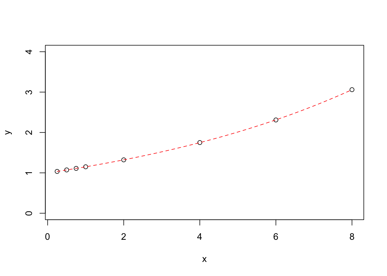 (The dotted line is \(1.15^x\) as produced by computer.)
Here, 1/8.4 = \(e^{-t/8267}\). So, \(e^{t/8267}\) = 8.4. Looking at the LL3 scale, we can see that the value of \(x\) where \(e^x\) = 8.4 is at a value of about \(x\) = 2.13 which we read on the D scale. Moving the right index of C to this number, we can move the cursor to about 8267 thus multiplying the two (within factors of 10); the result will be about 17,500 years. Practice those decimal points!
To find \(\sinh(1.73)\) we need \(e^{1.73}\) and \(e^{-1.73}\). Setting the cursor to 1.73 on D, we can find these two values on LL1 and LL01; I get 5.64 and 0.177, respectively. Subtracting these two and dividing by two I get \(\sinh(1.73)\) = 5.463/2 = 2.73. By adding the same two values and dividing by two I get \(\cosh(1.73)\) = 5.817/2 = 2.91.
Find \((1.057)^{38}\) and multiply the result by 10,000. To do so, set the cursor at 1.057 on the LL1 scale, and move the right index of C under the cursor. Slide the cursor to 3.8 on the C scale. Since we slide to the left then \((1.057)^{0.38}\) will be on the LL1 scale under the cursor. So \((1.057)^{3.8}\) will also be under the cursor on the LL2 scale. And, \((1.057)^{38}\) will be on the LL3 scale: I get about 8.25. So, the final account balance is about $82,500. (True answer: \(8.21958\times 10^{4}\).)
To find \(0.95^{87}\) we can use the LL01 scale. Line up the cursor at 0.95 on the LL01 scale. Move the right index of C to the cursor. Move the cursor to 8.7 on the C scale. Since the cursor is moved to the left, it is now aligned with \((0.95)^{0.87}\) . So, we find \((0.95)^{8.7}\) on the LL02 scale. Our desired answer, \((0.95)^{87}\), is on LL03: \((0.95)^{87}\) = 0.0115.
Unfortunately slide rules do not add results. So, we must make a table of values and add them up afterward. Lucky for us, though, the problem here can be simplified just a bit. Rewrite the infinite series as \[ f(x) = \frac{x^2}{4-x^2} = \frac{x^2}{4} + \frac{x^4}{4^2} + \frac{x^6}{4^3} + \ldots \\ = \left(\frac{x}{2}\right)^2 + \left(\frac{x}{2}\right)^4 + \left(\frac{x}{2}\right)^6 + \ldots \] and then just look up the various powers for (1.05/2). Start by setting the cursor to 1.05 on the D scale. Move 2 on C to 1.05 on D. Move the cursor to the index of C to read the result – 0.525 – on D. Find 0.525 on the LL02 scale and move the index of C to this number using the cursor. Then, lining up the cursor successively with 2, 4, 6, … , you can read the values of the various terms on the LL03 scale. (It must be on the LL03 scale because (a) we are looking to the left of the original number, and (b) the result will be smaller than 0.525 since it is being raised by a positive power.) Here is a table of the numbers I find for the first four terms of the series:
0.276
0.076
0.021
0.006
0.002
and adding up the results by hand (yes, I know…) I get \(f(1.05)\) = 0.381.
To estimate the natural logarithm of 11,458, we find this number on the LL3 scale and move the cursor there. Reading off of the D scale, I see 9.35 telling us that \(e^{9.35}\) is about 11,458. Thus, 9.35 is approximately the natural logarithm of 11,458. By computer: \(\ln(11458)\) = 9.3464435.
Tom Wyman and Robert Ones, “An Update on Log-Log Slide Rules Before 1910”, Jour. Oughtred Soc., V17 No1, pp 11-15 (2008).↩︎
Ibid.↩︎
Bob Otnes, “Log Log Scales”, Jour. Oughtred Soc. 1.1 p19 (1992), and “Log Log Scales – Revisted”, Jour. Oughtred Soc. 4.1 p9 (1995).↩︎
Ibid.↩︎
By “re-index”, we mean exchange the “1” at the left end of the C scale with the “1” at the right end of the C scale. In this example, we move the right index of C to the value of 1.35 on the LL2 scale.↩︎