3 Slide Rule ABC’s and D’s
Slide rules consist of sets of logarithmic scales that are used to add logarithms of numbers in order to perform multiplication and division, as well as other quick calculations. As described in our previous chapters, adding distances on the rule can be equated to adding logarithms of numbers. And now that logarithms are understood and the values of common logarithms \((\log x = \log_{10} x)\) can be readily computed, creating a logarithmic scale is straightforward. For instance, if one wanted to make a logarithmic scale that was 10 inches in length, where “1” was on the left end and “10” was on the right end, then a mark for the number \(x\) would be placed at a distance of (10 inches)\(\times \log x\) from the left-hand side: the “2” mark would be placed (10 inches)\(\times \log 2\) = 3.01 inches from the left end, the “4.5” mark would be placed (10 inches)\(\times \log 4.5\) = 6.532 inches from the left end, and so forth for any number one wants to mark on the rule. The last mark would be at (10 inches)\(\times \log 10\) = 10 inches as desired.
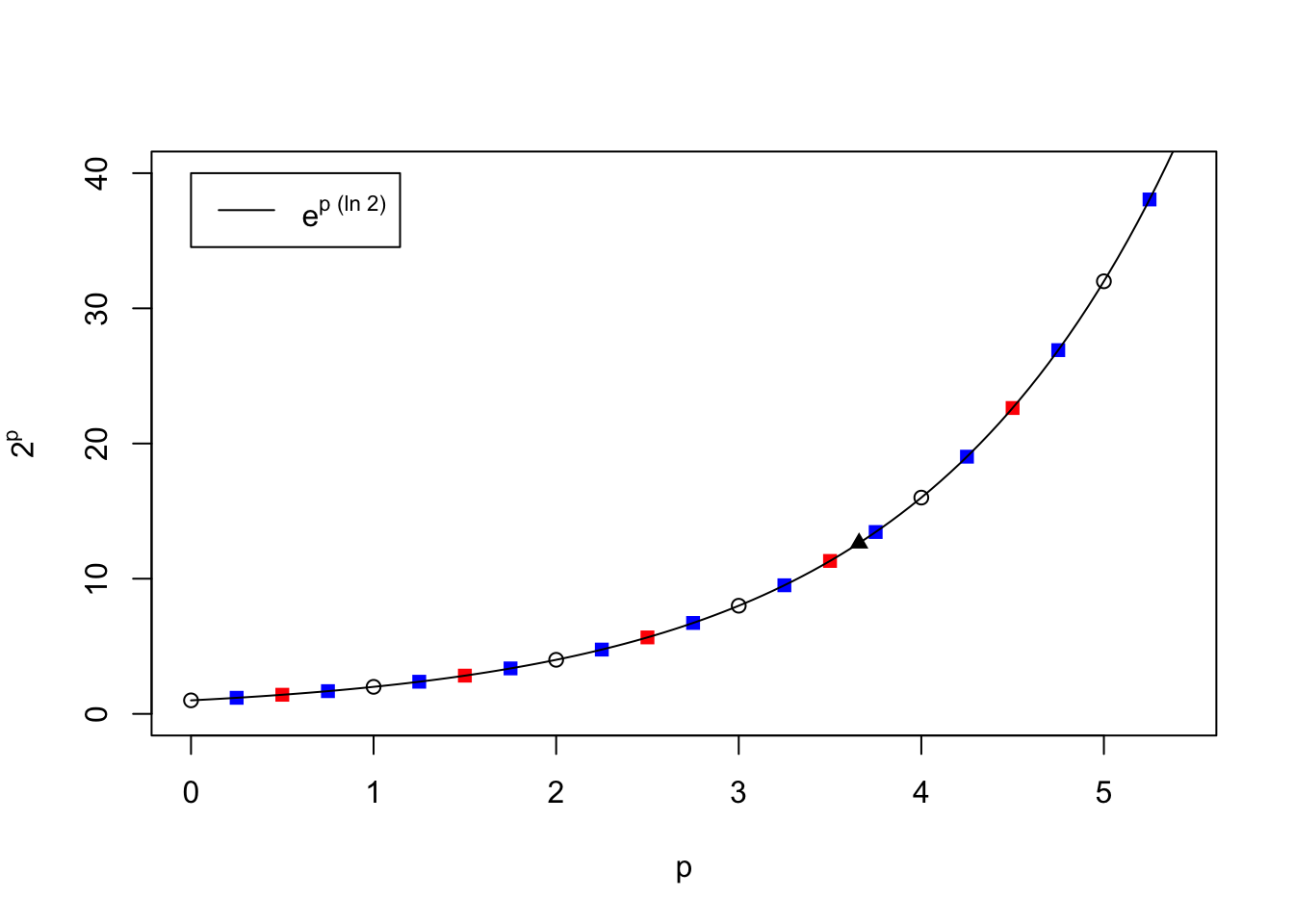
To get a feel for how to read the scales, some example numbers are indicated in the above figure by the red lines at values of 1.13, 1.65, 3.8, 7.1 and 9.6. As was discussed in Review of the Logarithm, if we created a scale like the one in the above figure but went between values of 10 to 100, or perhaps between values of 0.1 to 1, the spacing of the marks on the scale would be the same. Hence, the red lines could in principle represent values of 11.3, 16.5, 38, 71 and 96, or 0.113, 0.165, 0.38, 0.71 and 0.96 as well, depending upon the interpretation of the values of 1 and 10 at the left and right ends, respectively.
Edmund Gunter of England is credited as having made the first straight logarithmic scale of this kind in 1620, with which he used “dividers” (compasses) to measure and add up logarithms to perform calculations. In 1624, William Oughtred, also of England, arranged two Gunter rules and slid them back and forth (holding them together by hand) to do the same calculations without having to “measure” anything with dividers. Over the next several years devices were created to hold these sliding rules together, and circular variations of the basic design were created as well, even by Oughtred himself. It took over a century before cursors were added as an aid for lining up and reading results more accurately, particularly on instruments with more than two scales.
Without going through all the variants of the slide rule over these first two centuries following its invention, we’ll simply go directly to the standard Mannheim-style rule, introduced by Amédée Mannheim of France in about 1850. The Mannheim rule has four basic logarithmic scales, most often labeled A, B, C, and D. An example of such a rule is shown below.
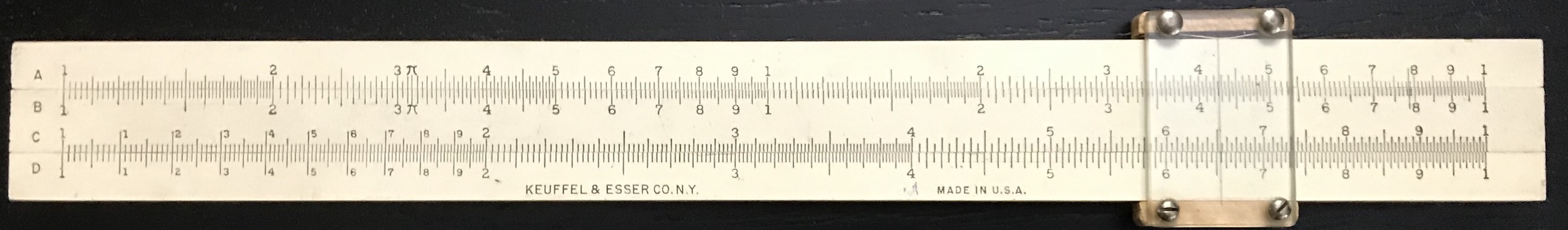
Notice that each scale has a layout similar to that created above. This is our standard “logarithmic scale”. The A and B scales are identical to each other, and the C and D scales are again identical to each other. The C/D scales cover one complete factor of 10, while the A/B scales have the same logarithmic scale pattern but is repeated and hence cover a factor of 100. This will be important later. On the particular rule shown and on many others, the A/B scales are labeled from 1 to 1 (interpreted as from 1 to 10), then 1 to 1 again (interpreted as from 10 to 100); on some slide rules “1, 2, …10” and “20, 30, …100” are written out explicitly.
The Mannheim scale layout and its labeling became standards that lasted over the remaining lifetime of the slide rule industry. These are the basic scales used for calculations involving multiplication, division, and for finding squares and square roots. The other scales we will discuss below are on many slide rules, but these four are found on essentially every standard slide rule.