4 Introduction to Rmarkdown

The purpose of this and the following chapters is to introduce the syntax and techniques used to produce nice-looking web pages using Rstudio and bookdown. By reading the relevant *.Rmd files that created the text you are reading, hopefully this will give you a head start in making your own online book-style web site.

For learning some of the basics of writing simple programs in R – particularly computational examples – see this online tutorial.

You can label chapter and section titles using {#label} after them, e.g., we can reference Chapter 4. If you do not manually label them, there will be automatic labels anyway, e.g., Chapter R and Rstudio.

Figures and tables with captions will be placed in figure and table environments, respectively.

x = c(0,2,5,7,9,12,21,32)
y = x^2
plot(x,y, type = 'b', pch = 19)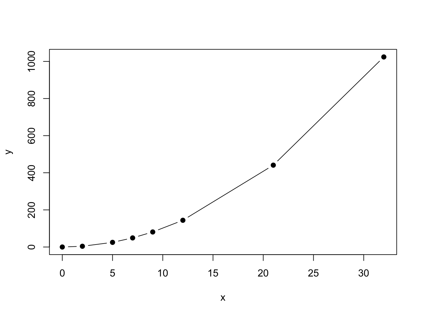

Figure 4.1: Here is a nice figure!

Reference a figure by its code chunk label with the fig: prefix, e.g., see Figure 4.1. Similarly, you can reference tables generated from knitr::kable(), e.g., see Table 4.1.

knitr::kable( 
  cbind(x,y), 
  caption = 'Here is a nice table!',
  booktabs = TRUE
)

Table 4.1: Here is a nice table!

x	y
0	0
2	4
5	25
7	49
9	81
12	144
21	441
32	1024

You can write citations, too. For example, we are using the bookdown package (Xie 2021) in this sample book, which was built on top of R Markdown (Allaire et al. 2021) and knitr (Xie 2015).